FT1. Final practice: stuck-at faults, scan, reliability and minimum energy

This page practises the final’s questions on testing chips and on running them at the lowest possible supply: how a tester finds one broken node through a scan chain and which bit out reveals it; why some chips die early and how burn-in catches them; how low a subthreshold supply can go, and whether some supply minimizes a chain’s energy. Every past-final part on these topics is here, re-solved from the papers; the keys’ answers are not copied, and where a key slips the page says so. The parts come in three families: stuck-at faults and scan (FN10-3, FN17-4a–b, FN19-4, PS5-Q3), clock latency and reliability short answers (FN17-1d, FN17-1e) and the lowest working supply and minimum energy (FN10-2c, FN17-10c). Each family opens with a How to approach section that gives the model and the moves once, and ends with harder added variations: longer chains, setups no past paper uses, and heavier arithmetic, as the real Fall 2026 midterm was.

Every part is worked the same way: what it asks, the idea, why this formula, the solution in steps (each gives its reason first), a check by another route, the answer, and what to remember. Try each part first; open the Hint if you are stuck. The answer key’s verdict is folded at the end of each past-paper part.

Before you start. Everything here is taught in Chapter 22 (scan, stuck-at faults, burn-in) and Chapter 23 (clock latency, electromigration, the low-voltage limit and minimum energy), on the device model of Chapter 4 and the energy of Chapter 6. Each section below restates what it uses:

• the scan flip-flop and the chain (Chapter 22 §4); the scan test and its bit order (§5); the waveforms (§5);
• the stuck-at model (§6); controllability and observability (§7), with reconvergent fan-out (§7); a fault through a chain end to end (§8);
• the master–slave flip-flop and the static latch (Chapter 13 §10, §8); the transmission-gate multiplexer (Chapter 10 §7); hold and skew (Chapter 14 §2);
• the bathtub curve and burn-in (Chapter 22 §10–§11); electromigration and its limits (Chapter 23 §3–§4); clock skew, jitter and latency (Chapter 23 §6);
• subthreshold current (Chapter 4 §11); the subthreshold chain’s current and delay, FN17-10a–b and FN10-2a–b (FN2); the functional limit and the minimum-energy supply (Chapter 23 §15–§16).

Conventions on this page.

• Fault values are written good/faulty: “0/1” means 0 in the good circuit and 1 in the faulty one. ST0 and ST1 are stuck at 0 and stuck at 1, at the node’s stem: every gate the node feeds sees the stuck value.
• Patterns list the inputs in the order the part names them, first bit first: “011” for $W_1W_2W_3$ means $W_1 = 0$0, $W_2 = W_3 = 1$1.
• Scan chains run scan_in → $F_1$ → … → $F_n$ → scan_out unless a part says otherwise. “Load”, “capture” and “unload” edges are the rising clock edges of the three phases; L1, C, U1 name them.
• Subthreshold numbers use the papers’ values: $S$ = 80 mV/decade, $I_{off}$ = 10 nA, and $kT/q$ = 26 mV. $\log$ is base 10 and $\ln$ natural; $10^{-V/S} = e^{-u}$ with $u = V\ln 10/S$Vln10/S.
• Pages are the papers’ printed page labels.

Symbols

Symbol	Meaning	Unit	First appears
ST0, ST1	a node stuck at 0, at 1	—	approach 1
$q_i$qi​, $W_i$	flip-flop $F_i$‘s output (the papers name some $W_i$Wi​)	—	approach 1
$D_i$Di​, $Y_i$	the logic’s output into flip-flop $F_i$‘s D input (FN17-4 names them $Y_i$Yi​)	—	approach 1
SE, SI	scan enable and scan in, a scan flip-flop’s extra inputs	—	approach 1
$n$	flip-flops in a scan chain	—	approach 1
$p$	test patterns	—	approach 1
$X$	the fault site in FN10-3 and FN19-4	—	FN10-3
$P$P, $Q$Q, $N_1$N1​, $N_2$	FN10-3’s internal nodes (this guide’s names)	—	FN10-3
$A$A, $Z_1$Z1​, $Z_2$Z2​, $X_1$	FN17-4’s fault site, primary outputs and primary input	—	FN17-4
$m$	the scan flip-flop’s mux output (PS5-Q3)	—	PS5-Q3
$t_L$	a clock network’s latency, root to leaf	ps	approach 2
$S_V$	the supply sensitivity of delay, $(V_{DD}/t)\,\partial t/\partial V_{DD}$	—	approach 2
$J$	current density, current over cross-section	mA/µm²	approach 2
$w$w, $w_{neck}$wneck​, $t$	a wire’s width, its width at a neck, its thickness	µm	approach 2
$S$	the subthreshold slope	mV/decade	approach 3
$kT/q$	the thermal voltage, 26 mV	mV	approach 3
$I_{off}$Ioff​, $I_{on}$	a device’s current at $V_{GS} = 0$ and at $V_{GS} = V_{DD}$	nA	approach 3
$V_{fn}$	the lowest supply at which the inverter still gives a 10–90 % swing	mV	approach 3
$C$	the capacitance on each node of a chain	fF	approach 3
$N$N, $N_g$Ng​, $\alpha$	logic depth, gates in the block, fraction of nodes that rise per operation	—	approach 3
$E$E, $E_{dyn}$Edyn​, $E_{leak}$	energy per operation, its switching and its leakage parts	fJ	approach 3
$T$	the time one operation takes (the chain’s delay)	ns	approach 3
$u$u, $K$	the supply in units of $S/\ln 10$S/ln10; the depth-to-activity number $N/(4\alpha)$	—	approach 3

How to approach a stuck-at or scan-test question

Recognize it by the words: “stuck-at-one (zero) fault at node …”, “test pattern”, “detect”, “propagate it to the output”, “is this pattern unique?”, “controllability and observability”, “scan in”, “scan_enable”, “in what order”, “scanned out”, “good” and “bad” circuit, “sketch the waveforms for scan_enable, clock, scan_in and scan_out”. The paper prints a gate network, often behind a chain of scan flip-flops (boxes with D, Q, SI, SE and a clock), and marks one node.

The model. A manufacturing defect is modelled as one node stuck at 0 or 1 (Chapter 22 §6). A pattern detects the fault when some observed output of the good circuit differs from the faulty one’s. Scan makes every flip-flop’s state an input the tester sets (shift in) and every flip-flop’s D an output it reads (shift out), so a sequential chip is tested as combinational logic, one pattern at a time (§5).

The scan chain in its two modes (Chapter 22 §4): with SE = 1 the flip-flops form a shift register from scan_in to scan_out; with SE = 0 each takes its D from the logic. Original figure ↗

A stuck-at testadded

$$\begin{aligned} \text{control:}\quad & \text{node} = \overline{\text{stuck value}}\ \text{(good circuit)}\\ \text{observe:}\quad & \text{side inputs} = \text{non-controlling}\\ & \text{(1 for AND/NAND, 0 for OR/NOR)} \end{aligned}$$

Holds when: a single stuck-at fault in combinational logic (with scan, the flip-flops' states are inputs and their D's are outputs); side inputs are set by working back to inputs the pattern controls

Scan order and test lengthadded

$$\begin{aligned} \text{scan\_in, in time order:}\quad & q_n,\ q_{n-1},\ \ldots,\ q_1\\ \text{scan\_out, in time order:}\quad & D_n,\ D_{n-1},\ \ldots,\ D_1\\ \text{edges for } p \text{ patterns:}\quad & p\,(n + 1) + n \end{aligned}$$

Holds when: a chain scan_in → F1 → … → Fn → scan_out, SE = 1 for shifting; scan_out is Fn's Q; the next load overlapped with the unload

Why these, and their conditions. Control: if the good node already sits at the stuck value, nothing can differ downstream. Observe: a gate passes a change on one input only if every other input is non-controlling (Chapter 22 §7). Memorize both. The order: derive it from one shift edge, which moves every bit one place along, so the first bit in travels farthest; scan_out is $F_n$‘s Q, so $D_n$ is readable right after the capture edge (§5). The count: $n$ load edges and one capture per pattern (the next load overlaps this unload), and $n$ more to empty the chain.

Reconvergent fan-out. When the fault site feeds two paths that meet again, the difference arrives on both, and the meeting gate decides: if the faulty value on a branch is the meeting gate’s controlling value, the good circuit must have every branch open for the outputs to differ; at an XOR, two open branches cancel and exactly one must be open (§7). The safe move is always the same: write good/faulty values on both branches and evaluate the meeting gate in each circuit.

The moves.

1. Write each node as a function of the inputs the pattern sets (flip-flop outputs and primary inputs). Name the internal nodes.
2. Control: set the fault site to the opposite of its stuck value; work back to the inputs.
3. Observe: pick a path to an observed output (a flip-flop’s D or a primary output); give every side input its non-controlling value; work back. Where the path reconverges, evaluate both branches.
4. Check the pattern by evaluating the good and the faulty circuit at every output. Count the patterns if the paper asks “unique?”: multiply the free inputs’ choices.
5. Scan it: list the load in chain order and reverse it for scan_in; capture with SE = 0 and the primary inputs applied; list the captured $D$‘s in chain order and reverse them for scan_out. Say which bit out first differs.

Decide on the way: which outputs are observed (through the chain, or as primary outputs); whether the paper wants the register view (the captured $D_1 \ldots D_n$D1​…Dn​) or the scan_out sequence (the same bits reversed); and which observation path makes the arithmetic shortest.

Traps. A side input left at its controlling value. Sensitizing one branch of a reconvergence where both are needed (FN10-3), or both where one is needed (an XOR). Reversing the load order. Reading the register view as the scan_out sequence. Forgetting that a primary input is applied by the tester during capture, not scanned in. Answering “unique?” without counting.

Playbook card: stuck-at faults and scan, with the scan flip-flop for PS5-Q3a.

FN10-3: a stuck-at-1 test through reconvergent fan-out (10 points)

You need

The stuck-at model (Chapter 22 §6). A fault is one node held at 0 or 1 whatever its gate tries to drive; a pattern detects it when an observed output differs between the good circuit and the faulty one. Values are written good/faulty.

Controlling values (Chapter 22 §7). A 0 on any input fixes an AND’s output at 0 and a NAND’s at 1; a 1 on any input fixes an OR’s output at 1 and a NOR’s at 0. With every other input at the non-controlling value (1 for AND/NAND, 0 for OR/NOR) the gate’s output follows the remaining input, inverted for NAND and NOR.

Reconvergent fan-out (Chapter 22 §7). When a node feeds two paths that meet at a later gate, the fault reaches that gate on every branch the pattern opens; evaluate both branches in both circuits.

Chapter 22’s reconvergent example (§7): there an AND joins the branches and one open branch is enough. In FN10-3 the joining gate is a NAND fed by two NORs, and the answer is the opposite. Original figure ↗

The question (FN10-3, p5, in the paper’s words). Determine a test pattern to detect a stuck-at-one fault at node X in the following network and propagate it to the output Z. Is this pattern unique? (10 points)

FN10-3’s network (Final 2010, p5, redrawn). The question calls the output Z; the figure labels it Y, and this page writes Y. The small labels $P$ and $Q$ (the outer ANDs’ outputs) and $N_1$N1​, $N_2$ (the NORs’ outputs) are this page’s; the key’s two handwritten 0s are in the exam’s figure below.

The exam’s own figure (FN10-3, p5)

FN10-3, p5 (source figure). The two handwritten 0s, on the outer ANDs’ outputs, are the key’s.

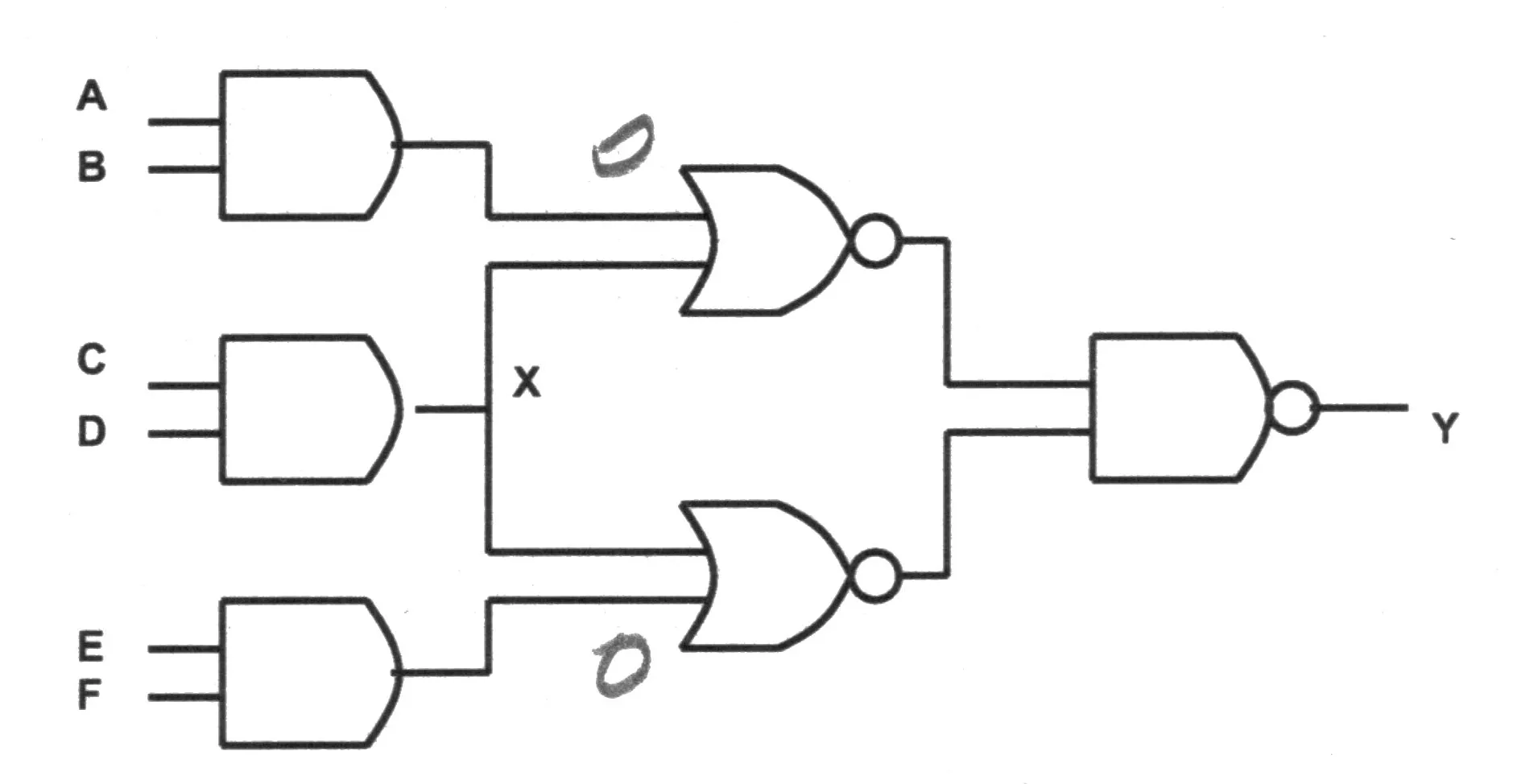
Reading the figure. $P = AB$AB, $X = CD$ and $Q = EF$ are ANDs. $X$ fans out to both NORs: $N_1 = \overline{P + X}$ and $N_2 = \overline{X + Q}$X+Q​. The NAND gives $Y = \overline{N_1 N_2}$N1​N2​​. So the two branches from $X$ reconverge at the NAND.

The pattern and whether it is unique (10 points)

FN10-3, p5. Determine a test pattern to detect a stuck-at-one fault at node X in the following network and propagate it to the output Z. Is this pattern unique? (10 points)

Hint

With X stuck at 1, what do both NORs output in the faulty circuit, whatever the other inputs are? What must the good circuit’s Y be, then?

What it asks. An input pattern $ABCDEF$ for which the good and the faulty networks give different $Y$Y, and whether only one such pattern exists. The words that decide the method are “detect” and “propagate it to the output”: control $X$ to 0, then carry the difference through the NORs and the NAND. “Unique?” asks for a count.

The idea. Control is easy ($CD \ne 11$CD=11); the difficulty is the reconvergence. In the faulty circuit $X = 1$ reaches both NORs, and 1 is a NOR’s controlling value, so the faulty $Y$ is 1 for every pattern. The good $Y$ must be 0, which needs both NORs at 1: the pattern must open both branches at once. The usual single-path recipe fails here.

Why this formula. Control ($X$X = opposite of 1) and observe (side inputs non-controlling) from Chapter 22 §7, applied to both branches.

• Where it comes from. A NOR passes a change on one input only if its other input is 0 (non-controlling). So $N_1$ follows $X$ inverted only when $P = 0$0, and $N_2$ only when $Q = 0$0. A NAND passes a change on one input only if the other is 1.
• Why both branches here. The faulty value 1 on each branch is the NOR’s controlling value, so both NOR outputs fall to 0 in the faulty circuit; the NAND sees 0 on both inputs. The good circuit must give the NAND 1 on both inputs, which needs both NORs open. In Chapter 22’s AND-joined example one branch sufficed because the steady branch sat at the AND’s non-controlling 1; here a steady branch would sit at 0, the NAND’s controlling value.
• A shortcut by algebra. $Y = \overline{N_1N_2} = (P + X) + (X + Q) = AB + CD + EF$EF, and the faulty $Y$ is 1, so the fault is detected exactly when $AB = CD = EF = 0$0.
• The tempting alternative. Sensitizing one path, say through $N_1$ with $P = 0$0, and leaving $E$E, $F$ free. With $E = F = 1$1, $Q = 1$ pins $N_2$ at 0 in both circuits, and $Y = 1$ in both: no detection.

FN10-3

1. Write the network. Because the outer gates are ANDs and the middle ones NORs, $P = AB$AB, $X = CD$CD, $Q = EF$EF, $N_1 = \overline{P + X}$P+X​, $N_2 = \overline{X + Q}$X+Q​, and $Y = \overline{N_1N_2} = AB + CD + EF$EF.
2. The faulty circuit. Because $X$ is stuck at 1 and 1 controls a NOR, $N_1 = N_2 = 0$ for every pattern, and $Y = \overline{0\cdot 0} = 1$1. The faulty output is 1 whatever the inputs.
3. Control. Because the good $X$ must be 0 (the opposite of its stuck value), $CD \ne 11$11: $C = 0$ or $D = 0$0. Now $X$ = 0/1.
4. Both branches. Because the good $Y$ must be 0 (the faulty one is 1), the NAND needs both inputs at 1: $N_1 = \overline{P + 0} = 1$ needs $P = AB = 0$0, and $N_2 = 1$ needs $Q = EF = 0$0. Now $N_1$ = 1/0, $N_2$ = 1/0, $Y$ = 0/1.
5. A pattern. Because every pair only has to avoid 11, the simplest is all zeros: $ABCDEF$ = 000000. Good: $P = X = Q = 0$0, $N_1 = N_2 = 1$1, $Y = 0$0. Faulty: $Y = 1$1. Detected.
6. Unique? Because each of the three pairs $AB$AB, $CD$CD, $EF$ may be any of 00, 01, 10, there are $3 \times 3 \times 3 = 27$ detecting patterns of the $2^6 = 64$64. Not unique; exhaustive simulation of both circuits finds exactly these 27.

FN10-3’s two patterns (new figure; good/faulty values from the fault simulation in checks.test.ts; thick: where the difference travels). (a) $ABCDEF$ = 000000 opens both branches, and $Y$ = 0/1: detected. (b) 110000 opens only the lower branch: $P = 1$ holds the upper NOR at 0 in both circuits (✗), the NAND sees a 0, and $Y$ = 1/1: not detected.

Check. By the one-branch counterexample: $ABCDEF$ = 110000 opens the lower branch ($Q = 0$Q=0, $X$ = 0/1, $N_2$ = 1/0) but $P = 1$ holds $N_1$ at 0 in both circuits, so $Y = \overline{0 \cdot N_2} = 1$ in both: not detected, as step 4 predicts. By fault equivalence: $P$ stuck at 1 and $N_1$ stuck at 0 also force $Y = 1$1, so they are detected by the same 27 patterns, and simulation agrees; $X$ stuck at 0, by contrast, needs $CD = 11$ with $AB$ and $EF$ free of 11, $1 \times 3 \times 3 = 9$ patterns.

Answer: for example $ABCDEF$ = 000000 (any pattern with $AB \ne 11$11, $CD \ne 11$ and $EF \ne 11$11): the good output is 0, the faulty output 1. It is not unique: 27 of the 64 patterns detect the fault. Both branches from $X$ must be sensitized, because the faulty 1 on either branch already forces the NAND’s output.

Remember. At a reconvergence, evaluate both branches in both circuits before choosing side inputs. When the faulty value is the controlling value of the gates it enters, the good circuit must open every branch. “Unique?” is a count: multiply the choices of the free inputs.

The answer key agrees

The key marks the outer ANDs’ outputs 0 (on the figure), sets $X = 0$ through $C$ or $D$D, and answers that the pattern is not unique, with both NOR paths sensitized. It does not count the patterns; the count is 27.

FN17-4: a stuck-at-0 fault behind a three-flip-flop scan chain (20 points)

You need

The scan flip-flop and the chain (Chapter 22 §4). Each flip-flop has a 2:1 multiplexer in front of D: at each rising clock edge $Q^+ = \overline{SE}\cdot D + SE\cdot SI$SI. With SE = 1 the flip-flops form a shift register; with SE = 0 each captures its D from the logic.

The scan test and its order (Chapter 22 §5). Shift in with SE = 1 (the last flip-flop’s value first), capture once with SE = 0 and the primary inputs applied, shift out with SE = 1. scan_out is the last flip-flop’s Q, so it shows that flip-flop’s captured value right after the capture edge, then the one before it after each shift.

Building the pattern (Chapter 22 §7–§8). Control the node to the opposite of its stuck value; give every side input on a path to an observed output its non-controlling value (1 for AND/NAND, 0 for OR/NOR).

The question (FN17-4, p9, in the paper’s words). Consider the circuit shown below.

FN17-4’s scan chain (Final 2017, p9, redrawn): scan_in → $F_1$ ($W_1$W1​) → $F_2$ ($W_2$W2​) → $F_3$ ($W_3$W3​) → scan_out, all on one clk and one scan_enable. The labels $F_1$–$F_3$ are this page’s. The box is the combinational logic (the paper’s “Comb. Logic”): its outputs $Y_1$Y1​, $Y_2$Y2​, $Y_3$ return to the flip-flops’ D inputs; $Z_1$Z1​, $Z_2$ are primary outputs and $X_1$ a primary input.

The exam’s own figure (FN17-4, p9)

FN17-4, p9 (source figure).

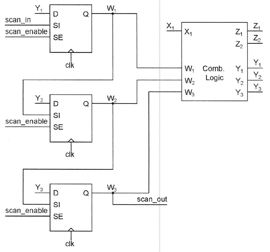
The block inside (FN17-4, p9, redrawn; the OR’s three inputs are spread wider than printed). $A$ is the paper’s name; this page names the OR’s output $O$ ($= Z_2 = Y_3$=Y3​). The key’s handwritten “ST0” at $A$ is in the exam’s figure below.

The exam’s own figure (FN17-4, p9)

FN17-4, p9 (source figure). The handwritten “ST0” at A is the key’s mark of the fault the parts ask about.

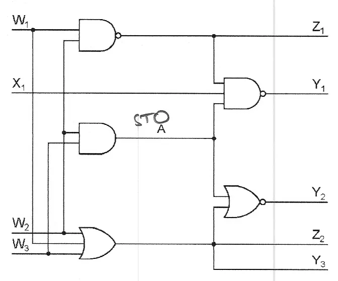
Reading the figure. From the wiring (checked on full-resolution crops): $Z_1 = \overline{W_1W_2}$W1​W2​​; $A = W_2W_3$W2​W3​; $O = W_1 + W_2 + W_3$W3​, which is both $Z_2$ and $Y_3$Y3​; $Y_1 = \overline{Z_1 \cdot X_1 \cdot A}$ (a three-input NAND); $Y_2 = \overline{A + O}$ (a NOR). The flip-flops hold $W_1$W1​, $W_2$W2​, $W_3$ and capture $Y_1$Y1​, $Y_2$Y2​, $Y_3$Y3​.

Part (a): the pattern and the order (10 points)

FN17-4a, p9. Determine an appropriate test pattern that achieves controllability and observability for a stuck-at-zero fault at node A. What value must be scanned into the flip-flops? In what order? (10 points)

FN17-4’s logic (p9): node $A$ feeds the NAND to $Y_1$ and the NOR to $Y_2$Y2​. Original figure ↑

Hint

Node A feeds two gates. Which of them can carry a change in A when A is 1, and what does the OR’s output do to the other?

What it asks. The flip-flop values $W_1W_2W_3$ (and the primary input $X_1$X1​) that make the good $A$ differ from the stuck 0 and carry the difference to an output the tester reads, and the time order in which those values go onto scan_in. “Controllability and observability” names the two conditions; “in what order” asks for the shift order.

The idea. Control first, because here it decides the observation path. Driving $A$ to 1 needs $W_2 = 1$1, which makes the OR’s output 1 and blocks the NOR to $Y_2$Y2​; only the NAND to $Y_1$ is left, and its side inputs fix the rest. Every input ends up forced: one pattern.

Why this formula. Control and observe (Chapter 22 §7) and the scan order “the last flip-flop’s value first” (§5).

• Where it comes from. A NAND passes one input only when all its other inputs are 1; a NOR only when its other input is 0. The order: each shift edge moves every bit one place toward scan_out, so the bit shifted in first ends in $F_3$F3​.
• Conditions. $X_1$ is not in the chain; the tester holds it at 1 through the capture edge. The capture is one rising edge with SE = 0. Single fault: only $A$ is wrong.
• The tempting alternative. Observing at $Y_2$ because the NOR is “closer”. The control condition $W_2 = 1$ makes the NOR’s side input 1, which blocks it. Also tempting: shifting in $W_1, W_2, W_3$ in that order, which loads them reversed.

FN17-4a

1. Control. Because $A = W_2W_3$ must be 1 in the good circuit (opposite to its stuck 0), $W_2 = W_3 = 1$1. Now $A$ = 1/0.
2. The NOR is blocked. Because $O = W_1 + W_2 + W_3 = 1$ once $W_2 = 1$1, and 1 controls a NOR, $Y_2 = 0$ in both circuits. No path through $Y_2$Y2​.
3. Observe through the NAND. Because $Y_1 = \overline{Z_1X_1A}$ passes $A$ only if $Z_1 = X_1 = 1$1: $X_1 = 1$ (primary input), and $Z_1 = \overline{W_1 \cdot 1} = 1$ needs $W_1 = 0$0. Now $Y_1$ = 0/1.
4. The pattern. $X_1 = 1$ and $W_1W_2W_3 = 011$011. Because every input was forced, it is the only detecting pattern of the 16 ($X_1W_1W_2W_3$X1​W1​W2​W3​); exhaustive simulation agrees, with or without $Z_1$ and $Z_2$ observed.
5. The order. Because the first bit shifted in ends in $F_3$F3​, scan_in carries $W_3$W3​, $W_2$W2​, $W_1$ = 1, 1, 0 on three rising edges with SE = 1. The chain then holds: after the first edge $F_1 = 1$1; after the second $F_1F_2 = 11$11; after the third $F_1F_2F_3 = 011$011.

Part (a)‘s pattern in the logic (new figure; good/faulty values computed): $X_1 = 1$1, $W_1W_2W_3 = 011$011. $A$ = 1/0 reaches $Y_1$ (thick) because the NAND’s other inputs, $Z_1$ and $X_1$X1​, are 1; at the NOR, $O = 1$ is controlling (✗), so $Y_2$ = 0/0.

Check. By the faulty circuit at that pattern: $A = 0$ makes $Y_1 = \overline{1 \cdot 1 \cdot 0} = 1$ against the good 0, while $Y_2 = 0$ and $Y_3 = 1$ in both: exactly one bit differs, as the path argument says. By trying the obvious alternative, $W_1 = 1$1: then $Z_1 = 0$0, a NAND’s controlling value, and $Y_1 = 1$ in both circuits. And by contrast with the opposite fault: $A$ stuck at 1 needs $A = 0$0, which many patterns give, and 6 of the 16 detect it.

Answer: scan $W_1W_2W_3 = 011$ into the flip-flops and hold the primary input $X_1 = 1$1. In time order scan_in carries 1, 1, 0 ($W_3$W3​ first, $W_1$ last). The fault is observed at $Y_1$Y1​; $Y_2$ cannot carry it, because $W_2 = 1$ makes the NOR’s other input 1. It is the only pattern that works.

Remember. Do control first; it often decides which observation path survives. A primary input in the logic ($X_1$X1​) is part of the pattern but is not scanned. To load $q_1 \ldots q_n$q1​…qn​, shift in $q_n$ first.

The answer key agrees

The key writes “Must control A to 1 ⇒ $W_2 = 1$1, $W_3 = 1$1. Must observe A at output $Y_1$ ⇒ $W_1 = 0$0, $X_1 = 1$1”, the same pattern. It answers “in what order?” only by listing $W_1 = 0$0, $W_2 = 1$1, $W_3 = 1$1; the order on scan_in is 1, 1, 0 ($W_3$W3​ first).

Part (b): what comes out, good and bad (10 points)

FN17-4b, p9. After the scanned pattern of (a) is clocked once, what values will be scanned out of the registers for the “bad” circuit? What would be expected values for the “good” circuit? (10 points)

FN17-4’s chain (p9): $F_3$‘s Q is scan_out, so $Y_3$ comes out first. Original figure ↑

Hint

After the capture edge, which flip-flop’s value is already on scan_out, and which comes next?

What it asks. The captured values $Y_1Y_2Y_3$ for the faulty and the good circuit, and how they leave the chain. “Clocked once” is the capture edge with SE = 0; “scanned out” asks for the sequence on scan_out.

The idea. One capture edge copies $Y_1$Y1​, $Y_2$Y2​, $Y_3$ into $F_1$F1​, $F_2$F2​, $F_3$F3​; evaluate them in both circuits. Shifting then brings them out from the scan_out end: $Y_3$ first, $Y_1$ last. The fault sits in $Y_1$Y1​, so it is the last bit out.

Why this formula. The capture rule $Q^+ = D$ at SE = 0, and scan_out in time order $D_n, D_{n-1}, \ldots, D_1$ (Chapter 22 §5).

• Where it comes from. scan_out is wired to $F_3$‘s Q, so after the capture edge it shows $F_3$‘s new value, $Y_3$Y3​; each unload edge moves $F_2$‘s value into $F_3$F3​, then $F_1$‘s.
• Conditions. SE = 0 for exactly one rising edge, then SE = 1. The register view and the scan_out sequence hold the same bits in reverse order; give both, labelled.
• The tempting alternative. Reporting $Y_1, Y_2, Y_3$ as “what is scanned out”: that is the register view, read backwards.

FN17-4b

1. The good circuit at $X_1 = 1$1, $W_1W_2W_3 = 011$011. Because $Z_1 = \overline{0\cdot1} = 1$1, $A = 1\cdot1 = 1$ and $O = 1$1: $Y_1 = \overline{1\cdot1\cdot1} = 0$0, $Y_2 = \overline{1 + 1} = 0$0, $Y_3 = O = 1$1. Captured $(Y_1, Y_2, Y_3) =$ (0, 0, 1).
2. The bad circuit. Because $A$ is stuck at 0: $Y_1 = \overline{1\cdot1\cdot0} = 1$1, $Y_2 = \overline{0 + 1} = 0$0, $Y_3 = 1$1. Captured (1, 0, 1).
3. Scan out. Because scan_out is $F_3$‘s Q, it reads $Y_3$Y3​, then $Y_2$Y2​, then $Y_1$Y1​: good 1, 0, 0; bad 1, 0, 1. The first two bits agree; the third differs.
4. The primary outputs. Because $Z_1 = 1$ and $Z_2 = O = 1$ do not depend on $A$A, they agree in both circuits; the fault is seen only through the chain.

Part (b) as waveforms (computed from the scan model’s cycle table; hatched: unknown or don’t care). Loading 1, 1, 0 sets $W_1W_2W_3 = 011$011. After the capture edge C, scan_out shows $Y_3 = 1$1, then $Y_2 = 0$ after U1 and $Y_1$ after U2: 0 in the good circuit, 1 with $A$ stuck at 0 (≠). The third bit out tells them apart.

Check. By symmetry of the two parts: in (a) the bit that goes in last, $W_1$W1​, ends nearest scan_in; in (b) the bit that comes out last, $Y_1$Y1​, is the one nearest scan_in. Both are $F_1$F1​, the flip-flop whose D carries the fault, so the fault must be the last bit out, as step 3 finds. By the fault itself: only $Y_1$ differs, consistent with (a)‘s single path.

Answer: after one capture edge the registers hold good $(Y_1, Y_2, Y_3) = (0, 0, 1)$ and bad $(1, 0, 1)$(1,0,1). Scanned out ($Y_3$Y3​ first), the good circuit gives 1, 0, 0 and the bad circuit 1, 0, 1: the third bit out, $Y_1$Y1​, reveals the fault.

Remember. Evaluate the captured $D$‘s in both circuits, then reverse them for scan_out. The bit that shows the fault comes out in the position of its flip-flop counted from scan_out.

The answer key agrees

The key writes $Y_1, Y_2, Y_3 \Rightarrow 0, 0, 1$ expected and $1, 0, 1$ bad, circling $Y_1$Y1​. It gives the register values and does not say in which order they leave the chain; on scan_out the order is $Y_3$ first: good 1, 0, 0 and bad 1, 0, 1.

FN19-4: scan waveforms for a stuck-at-1 fault (20 points)

You need

The scan test, cycle by cycle (Chapter 22 §5). With $n$ flip-flops: $n$ load edges with SE = 1, each taking one scan_in bit, the last flip-flop’s value first; one capture edge with SE = 0; then unload edges with SE = 1. SE changes between edges, a setup time before the next one. scan_out shows the last flip-flop’s capture right after the capture edge, and one more flip-flop’s capture after each unload edge.

Chapter 22’s three-flip-flop test as waveforms (§5): the layout FN19-4 asks for, with six flip-flops. Original figure ↗

Building the pattern (Chapter 22 §7). Control the fault site to the opposite of its stuck value; open a path to a flip-flop’s D with non-controlling side inputs.

The question (FN19-4, p9, in the paper’s words). Sketch the waveforms for scan_enable, clock, scan_in, and scan_out for a test sequence to scan in a test pattern, clock the system once, and scan out the resulting pattern such that a stuck-at-one fault at node X could be detected. Show where this would be detected in your waveform. (20 points)

FN19-4’s circuit (Final 2019, p9, redrawn; dots added at the junctions). This page numbers the flip-flops in chain order: $F_1$–$F_4$ down the left column, $F_5$ at the bottom right, $F_6$ at the top right (scan_out). It names the upper AND’s output $P = q_1q_2$q1​q2​; the lower AND’s output is the paper’s $X = q_3q_4$q3​q4​. $D_6 = \overline{P}$ and $D_5 = \overline{P + X}$P+X​. The left column’s D inputs come from logic outside the figure.

The exam’s own figure (FN19-4, p9)

FN19-4, p9 (source figure).

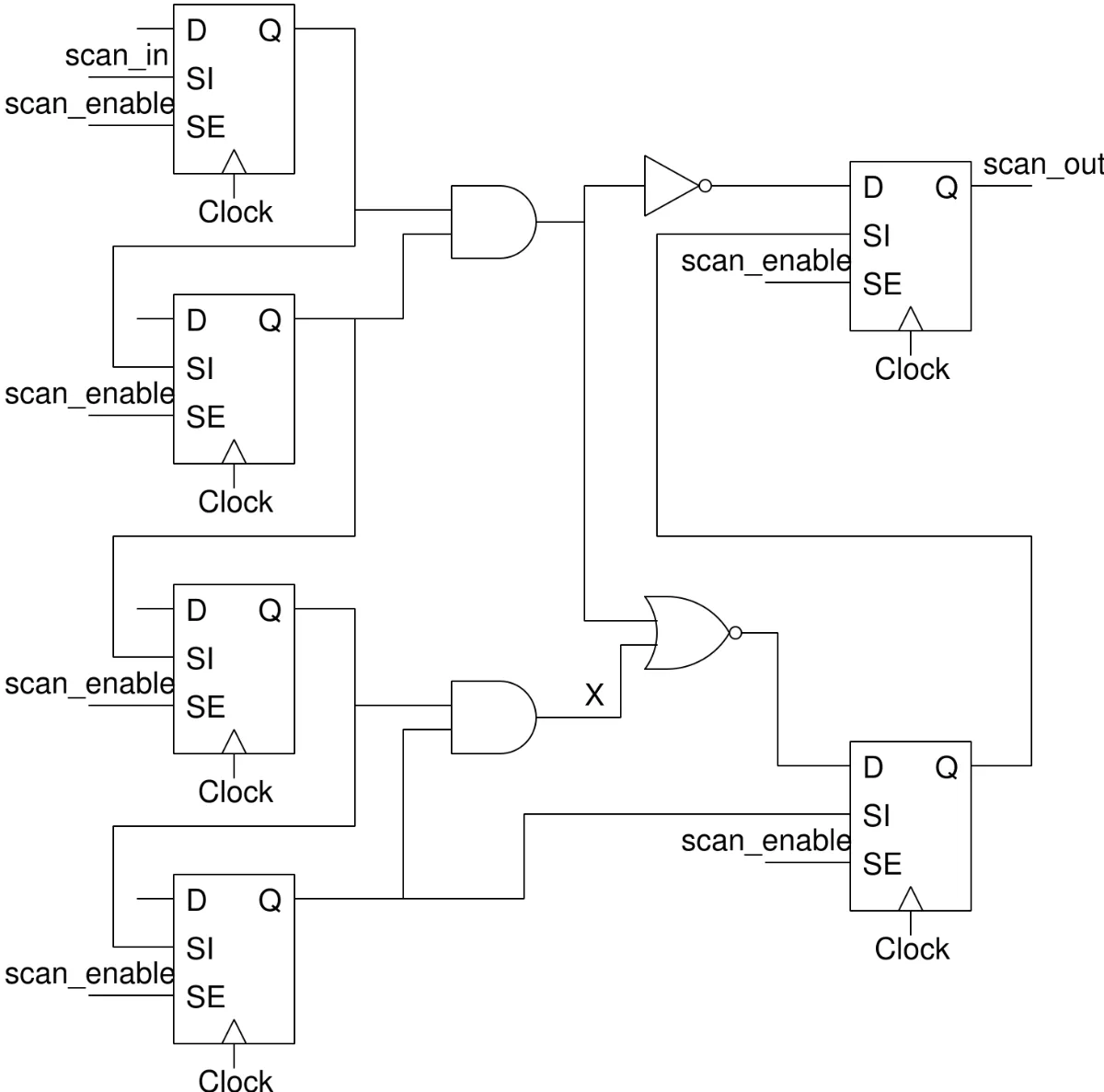
Reading the figure. Following each Q to the next SI gives the chain scan_in → $F_1$ → $F_2$ → $F_3$ → $F_4$ → $F_5$ → $F_6$ → scan_out: $F_4$‘s Q goes across to the bottom-right flip-flop’s SI, and that one’s Q up to the top-right one’s SI. The logic reads only $q_1 \ldots q_4$ and feeds only $F_5$ and $F_6$F6​.

The waveforms and where the fault shows (20 points)

FN19-4, p9. Sketch the waveforms for scan_enable, clock, scan_in, and scan_out for a test sequence to scan in a test pattern, clock the system once, and scan out the resulting pattern such that a stuck-at-one fault at node X could be detected. Show where this would be detected in your waveform. (20 points)

Hint

X feeds only the NOR into F5. What must the NOR’s other input be, and how many edges after the capture does F5’s value reach scan_out?

What it asks. Four waveforms on one time axis: SE, the clock, scan_in and scan_out, for a load, one capture and an unload, with a load that detects $X$ stuck at 1, and a mark at the bit where the good and faulty scan_out differ. The unknowns are the load (six bits), its order on scan_in, and the position of the detecting bit.

The idea. Solve the fault first, then draw the scan order in time. $X$ feeds only the NOR into $F_5$F5​, so the pattern must control $X$ to 0 and hold the NOR’s other input at 0; $q_5$q5​, $q_6$ are free. The waveforms are six load edges, one capture, and unload edges; $F_5$ is second from scan_out, so its bit, where the fault appears, is the second out.

Why this formula. Control and observe, and the scan order (Chapter 22 §5): scan_in in time order $q_6, q_5, \ldots, q_1$q6​,q5​,…,q1​; scan_out in time order $D_6, D_5, \ldots$D6​,D5​,….

• Where it comes from. Each shift edge moves every bit one place toward scan_out; scan_out is $F_6$‘s Q.
• Conditions. SE must be steady a setup time before each edge and a hold time after it, so it changes between edges, in the clock’s low phase. The left column’s captured values are not drawn by the paper (their D’s come from outside); draw them as unknown on scan_out.
• The tempting alternatives. Observing at $D_6$D6​: $D_6 = \overline P$ does not depend on $X$X. Unloading only one edge: that shows $D_6$ and $D_5$ only if scan_out is sampled after the edge; say where you sample.

FN19-4

1. Control. Because $X = q_3q_4$ must be 0 in the good circuit, $q_3q_4 \ne 11$11. Now $X$ = 0/1.
2. Observe at $D_5$D5​. Because $X$ reaches only the NOR, and the NOR passes it only if $P = q_1q_2 = 0$ (non-controlling), $q_1q_2 \ne 11$11. Then $D_5 = \overline{0 + X}$ = 1/0.
3. Choose a load. Because $q_5$q5​, $q_6$ are free, choose $q_1 \ldots q_6 = 101000$ (any of $3 \times 3 \times 4 = 36$ of the 64 loads works; all zeros is the simplest). Good: $P = 0$0, $X = 0$0, $D_5 = 1$1, $D_6 = 1$1. Faulty: $D_5 = 0$0, $D_6 = 1$1.
4. SE and the load. Because the first bit in ends in $F_6$F6​, scan_in carries $q_6, q_5, q_4, q_3, q_2, q_1$ = 0, 0, 0, 1, 0, 1 on the rising edges L1–L6, each bit steady around its edge, with SE = 1.
5. Capture. Because the logic must be captured once, SE falls after L6 and before the next edge, C, then rises again after C. At C: $F_5 \leftarrow D_5$D5​, $F_6 \leftarrow D_6$ ($F_1$F1​–$F_4$ take their outside inputs).
6. Unload and detect. Because scan_out is $F_6$‘s Q: right after C it shows $D_6$ = 1 in both circuits; after U1 it shows $F_5$‘s capture, $D_5$D5​: 1 good, 0 faulty. Mark the bit between U1 and U2. U2–U5 bring out $F_4 \ldots F_1$‘s captures (unknown); U6 completes the six-edge unload, so a tester that samples just before each edge reads $F_1$‘s bit there, while the next pattern shifts in. In all, 6 + 1 + 6 = 13 edges for one pattern.

FN19-4’s answer as waveforms (computed from the scan model’s cycle table; hatched: unknown or don’t care). scan_in carries $q_6 \ldots q_1$ = 0, 0, 0, 1, 0, 1, loading 101000. After C, scan_out shows $D_6 = 1$ in both circuits; after U1 it shows $D_5$D5​: 1 in the good circuit, 0 with $X$ stuck at 1 (≠). That is where the fault is detected. The later bits are $F_4 \ldots F_1$‘s captures, from logic off the figure.

Check. By counting from scan_out: $F_5$ is the second flip-flop from scan_out, so its captured value is the second bit out; $F_6$ (first bit out) carries $\overline P$P, which the fault cannot change. By the count: of the 64 loads, those with $q_1q_2 \ne 11$ (3 ways), $q_3q_4 \ne 11$ (3 ways) and any $q_5q_6$ (4 ways) detect: 36, which exhaustive simulation confirms; every one shows the fault at $D_5$ only.

Answer: load, for example, $q_1 \ldots q_6 = 101000$ (any load with $q_1q_2 \ne 11$ and $q_3q_4 \ne 11$11): SE high for six edges with scan_in 0, 0, 0, 1, 0, 1; SE low for one capture edge; SE high to shift out. scan_out shows $D_6 = 1$ in both circuits after the capture, then $D_5$D5​, 1 good and 0 faulty, after the first unload edge: the fault shows at the second bit out.

Remember. A waveform answer is the scan order drawn in time: SE high for $n$ edges, low for one, high again; scan_in reversed; scan_out reversed. Mark the bit by counting the faulty flip-flop’s position from scan_out.

The answer key agrees

FN19 has no official key. The unofficial proposed solution loads a pattern with $q_1q_2 \ne 11$ and $q_3q_4 \ne 11$ and finds the fault in $F_5$‘s bit, the second out after the capture, as here.

PS5-Q3: the scan flip-flop and the scan test

You need

The master–slave flip-flop (Chapter 13 §10). Two latches in series on opposite clock phases. Chapter 13’s drawing puts the master on clk (transparent while clk = 1), so it captures at the falling edge; swapping the phases (master transparent while CLK = 0, slave while CLK = 1) captures at the rising edge.

The master–slave flip-flop (Chapter 13 §10): swap clk and clk̄ for the rising-edge cell PS5 asks for. Original figure ↗

The static latch (Chapter 13 §8). A transmission gate lets D in while the latch is transparent; a feedback inverter and a second transmission gate, on the opposite phase, close the loop while it holds, so the stored value is driven, not just stored as charge: static.

The gated-feedback latch (Chapter 13 §8): the building block of each half. Original figure ↗

A 2:1 multiplexer (Chapter 10 §7). Two transmission gates with complementary selects: exactly one conducts, so the output follows one input.

The question (PS5-Q3, p3, in the problem set’s words). To improve the testability of a digital integrated circuit (that is, to improve the ability to detect and isolate manufacturing faults), it is a common practice in flop-based designs to modify the basic master-slave flip-flop (with inputs D, for data, CLK, for clock, and Q, for output) described in class to include two additional inputs, SI (for scan in) and SE (for scan enable). The function table for this “testability-enhanced” flip-flop is shown below:

D	SI	SE	CLK	Q[n+1]
1	X	0	rising edge	1
0	X	0	rising edge	0
X	X	X	falling edge	Q[n]
X	1	1	rising edge	1
X	0	1	rising edge	0

The table’s cell at gate level (Chapter 22 §4, Lecture21 @ 33:30): a 2:1 multiplexer on SE (input 0 is D, input 1 is SI) in front of a rising-edge flip-flop. X in the table means “don’t care”. Part (a) asks for the transistors inside.

Reading the table. Rows 1–2: with SE = 0 a rising edge loads D. Rows 4–5: with SE = 1 a rising edge loads SI. Row 3: a falling edge changes nothing. So $Q^{+} = \overline{SE}\cdot D + SE\cdot SI$ at each rising edge.

Part (a): the static scan flip-flop at the switch level

PS5-Q3a, p3. Draw the schematic for a static flip-flop enhanced in this way.

Hint

Which block selects between D and SI, and which edge must the master latch close on for the table’s rising-edge rows?

What it asks. A transistor-level circuit that behaves as the table says. “Static” decides the latch style: each latch must hold its value through a feedback loop, not on a floating node. “Master-slave flip-flop … described in class” decides the core: Chapter 13’s two latches, with the phases set for the rising edge.

The idea. Build it in two pieces: a 2:1 transmission-gate multiplexer on SE that feeds a node $m$m, then a static master–slave flip-flop on $m$m. For a rising edge the master is transparent while CLK = 0 and closes as CLK rises, when the slave opens; the slave closes when CLK falls, which is why a falling edge changes nothing (row 3). Each latch is Chapter 13 §8’s gated-feedback latch.

Why this formula. The cell’s function $Q^+ = \overline{SE}\cdot D + SE\cdot SI$SI, built from a multiplexer and a positive-edge flip-flop.

• Where it comes from. The multiplexer gives $m = \overline{SE}\cdot D + SE\cdot SI$ at all times; the flip-flop copies $m$ to Q at each rising edge (Chapter 22 §4).
• Why transmission gates. An NFET alone passes a weak 1 and a PFET alone a weak 0; the pair passes both rails (Chapter 10). The selects are complementary, so exactly one input drives $m$m.
• Conditions. SE, D and SI must be steady a setup time before the rising edge and a hold time after it; change SE while CLK is low, before the master has to settle. Two inversions between $m$ and Q (one per latch) make Q = $m$m; with an odd number, add an output inverter.
• The tempting alternative. Putting the master on CLK (transparent while CLK = 1), as Chapter 13’s drawing does: that flip-flop captures at the falling edge, against the table. Another: a dynamic latch (a transmission gate into an inverter with no feedback), which is not static.

PS5-Q3a

1. The multiplexer. Because D must pass while SE = 0, its transmission gate has its NFET on $\overline{SE}$ and its PFET on SE; SI’s gate is the mirror (NFET on SE, PFET on $\overline{SE}$SE). Their outputs join at $m$m: $m = \overline{SE}\cdot D + SE\cdot SI$SI.
2. The master latch. Because it must follow $m$ while CLK = 0 and hold when CLK rises, its input gate has its NFET on $\overline{CLK}$ and its PFET on CLK. A forward inverter drives the master’s output; a feedback inverter and a feedback gate on the opposite phase (NFET on CLK, PFET on $\overline{CLK}$CLK) close the loop while CLK = 1.
3. The slave latch. Because it must open when CLK rises and hold when CLK falls, its input gate has its NFET on CLK and its PFET on $\overline{CLK}$CLK, and its feedback gate the reverse. Its forward inverter drives Q.
4. The complements. Because the gates need $\overline{SE}$ and $\overline{CLK}$CLK, two inverters make them from SE and CLK.
5. The polarity. Because each latch has one forward inverter, $m$ is inverted twice on its way to Q: Q = $m$ at the rising edge, as the table needs.
6. The count. $2 \times 2$ (mux) $+ 2 \times 8$ (two latches, each two gates and two inverters) $+ 2 \times 2$ (the two complement inverters) $= 24$ transistors.

The scan flip-flop at the switch level (new figure, added). A multiplexer of two transmission gates (dashed box) passes D while SE = 0 and SI while SE = 1 to node $m$m. A static master–slave flip-flop follows: the master latch is transparent while CLK = 0 and the slave while CLK = 1, so Q takes $m$ at the rising edge. Each transmission gate is an NFET (gate label above) and a PFET (below) in parallel; the two inverters at the lower left make $\overline{SE}$ and $\overline{CLK}$CLK.

Check. By walking the table through the circuit. Row 1 (D = 1, SE = 0): while CLK = 0 the D gate conducts, $m = 1$ and the master follows it; at the rising edge the master closes on 1 and the slave opens: Q = 1. Row 4 (SI = 1, SE = 1): the same with SI. Row 3: when CLK falls the slave closes its loop and holds Q while the master reopens, so Q keeps its value. Chapter 22’s two-latch model of the cell, run edge by edge in this page’s test, gives the same rows. By the static test: in every phase each storage node is driven by an inverter through a conducting gate, so no node floats.

Answer: the circuit drawn above: a two-transmission-gate multiplexer (D passes while SE = 0, SI while SE = 1) into a static positive-edge master–slave flip-flop (master transparent while CLK = 0, slave while CLK = 1, each latch with switched feedback), plus inverters for $\overline{SE}$ and $\overline{CLK}$CLK: 24 transistors.

Remember. A scan flip-flop is a mux on SE in front of an ordinary flip-flop. For a rising-edge cell, the master is transparent while CLK is low. “Static” means a closed feedback loop in each latch while it holds.

The answer key agrees

PS5 has no official key. The agent-written solution in the course folder (a cross-check only) draws the same cell: a two-transmission-gate mux, a master transparent while CLK = 0 and a slave while CLK = 1, each latch with switched feedback, locally made $\overline{SE}$ and $\overline{CLK}$CLK, 24 devices. Its latches put two inverters in the forward path and close the loop with one gate, a variant of the same static latch.

Part (b): why scan helps, and the test procedure

PS5-Q3b, p3. With this type of flip-flop design it is possible to reconfigure all the flip-flops in the machine as a long shift register (called a scan chain), in which the output of each flip-flop is connected to the SI input of another. How might this improve our ability to test a chip? What would be the test procedure?

A three-flip-flop chain in its two modes (Chapter 22 §4). Original figure ↗

Hint

Without the chain, how would a tester put a chosen value into a flip-flop deep inside the chip, and how would it read one out?

What it asks. Two short answers: what the chain changes about testing, in the course’s terms (controllability, observability), and the steps a tester follows. No numbers are asked; a good answer names the three phases and says what each does.

The idea. A sequential circuit is hard to test because its state can be reached only by driving the machine through many cycles from its pins, and seen only through a few outputs. The chain turns every flip-flop into a test point: shifting in makes every state bit controllable, shifting out makes every captured logic output observable. The logic between flip-flops is then tested as combinational logic, with patterns computed for single stuck-at faults (automatic test pattern generation).

Why this formula. The shift rule ($Q^+ = SI$Q+= with SE = 1, so the chain is a shift register) and the capture rule ($Q^+ = D$Q+= with SE = 0); the test length $p(n + 1) + n$ edges for $p$ patterns on $n$ flip-flops.

• Where it comes from. $n$ edges load a chain of $n$n; one edge captures; the next load’s $n$ edges shift the result out at the same time; $n$ more edges empty the chain after the last pattern (Chapter 22 §5).
• Conditions. Each pattern targets the combinational logic between flip-flops. The chain itself must work, so it is tested first by shifting a known sequence straight through. Primary inputs are set by the tester during capture and primary outputs read then.
• The tempting alternative. “Functional testing”: run programs and check the results. The coverage of real defects is unknown and the time enormous; the lecture’s “test coverage ✗” (Chapter 22 §3).

PS5-Q3b

1. Why it helps: controllability. Because with SE = 1 the flip-flops form one shift register from scan_in to scan_out, any state can be loaded in $n$ clock edges, whatever logic sits between the flip-flops.
2. Why it helps: observability. Because one capture edge with SE = 0 copies every flip-flop’s D, and shifting brings every captured bit out, the response of every logic cone that ends in a flip-flop is read.
3. Why it helps: the problem shrinks. Because the state is now an input and the next state an output, only combinational logic remains; a mismatch’s position in the output stream also points to the flip-flop whose logic cone holds the fault.
4. The procedure. (i) Test the chain: shift a known sequence (for example alternating 0s and 1s) through with SE = 1 and check that it emerges $n$ edges later. (ii) For each pattern: with SE = 1, shift the pattern in ($n$n edges, the last flip-flop’s bit first). (iii) Set SE = 0, apply the primary inputs, give one clock edge to capture. (iv) Set SE = 1 and shift the response out ($n$n edges), comparing each bit with the good circuit’s response; shift the next pattern in at the same time. (v) Any mismatch fails the chip.
5. The cost, for example. Because one pattern takes $n + 1$ edges when loads and unloads overlap: a chip with 1,000 scan flip-flops and 500 patterns needs $500 \times 1001 + 1000 = 501{,}500$ edges, 5.015 ms at a 100 MHz scan clock; without the overlap, $500 \times 2001 = 1{,}000{,}500$1,000,500.

Check. By running the procedure on FN17-4 above: three load edges (1, 1, 0), one capture edge with $X_1 = 1$1, and two unload edges bring out the faulty bit; the first two bits out match the good circuit, as steps (iii)–(iv) say they must for a fault in $F_1$‘s cone. By the cost: per pattern, $n$ edges dominate, so test time grows with the chain length, which is why chips split their flip-flops into many short chains loaded in parallel (Variation 3).

Answer: the chain makes every flip-flop controllable (any state shifted in) and observable (every captured value shifted out), so the chip is tested as combinational logic with stuck-at patterns. Procedure: test the chain itself; then per pattern, shift in with SE = 1, capture once with SE = 0 and the primary inputs applied, shift out with SE = 1 (loading the next pattern) and compare.

Remember. Three phases: shift in, capture once, shift out. Name controllability and observability. Test length is about $p(n + 1)$ edges.

The answer key agrees

PS5 has no official key. The agent-written solution (cross-check only) gives the same benefits (controllability of the state, observability of the response, a combinational test) and the same procedure: check the chain with a known sequence, shift in with SE = 1, capture with SE = 0, shift out while loading the next pattern, compare.

Harder variations: stuck-at faults and scan

You need

A stuck-at test (Chapter 22 §7). Control the node to the opposite of its stuck value; give side inputs their non-controlling value (1 for AND/NAND, 0 for OR/NOR); at a reconvergence, evaluate both branches in both circuits. Through an XOR, exactly one branch may be open.

The scan order (Chapter 22 §5). scan_in carries the chain’s last flip-flop’s value first; scan_out shows the last flip-flop’s capture first. “Last” means last in the chain, whatever the flip-flops are named. A test of $p$ patterns on a chain of $n$ takes $p(n + 1) + n$ edges with overlapped loads.

Hold (Chapter 14 §2). Data launched at an edge must not reach the next flip-flop before that flip-flop’s hold time after the same edge: $t_{clk\to Q,\min} + t_{path,\min} \ge t_{hold} + \delta$δ, with $\delta$ the capturing clock’s lateness (skew).

The short path against skew (Chapter 14 §2): the race a scan link runs. Original figure ↗

These variations added are harder than the papers in the ways the real midterm was: Variation 1 puts an XOR reconvergence behind a chain wired out of numerical order, a five-step chain from fault to waveform; Variation 2 asks for coverage and a whole test set instead of one pattern; Variation 3 turns the chain into test time and a hold race, a setup no paper uses. The budgets assume the practice finals’ pace, about 1.8 minutes a point. No key exists, so there is no key verdict.

Variation 1: an XOR reconvergence behind a reordered chain (about 25 minutes)

Variation 1: an XOR reconvergence behind a reordered chain

added The question. Four scan flip-flops $F_1$–$F_4$ (outputs $q_1$–$q_4$q4​) are chained in layout order, scan_in → $F_3$ → $F_1$ → $F_4$ → $F_2$ → scan_out. A primary input $P$ and a primary output $Z$Z. The logic: $X = \overline{q_1q_2}$q1​q2​​; $a = X\cdot q_3$q3​; $b = \overline{X + P}$X+P​; $D_1 = a \oplus b$b; $D_2 = X + q_4$q4​; $D_3 = \overline{q_3q_4}$q3​q4​​; $D_4 = b\cdot q_1$q1​; $Z = \overline{a + q_4}$a+q4​​. Node $X$ is stuck at 1. (a) Write the good and faulty values of $a$a, $b$b, $D_1$D1​, $D_2$D2​, $D_4$ and $Z$ once $X$ is controlled. (b) How many of the 32 patterns $(q_1q_2q_3q_4, P)$ detect the fault? (c) For which $(q_3, P)$ does $D_1$ alone show it, and why does $q_3 = 1$1, $P = 0$ not? (d) Find a pattern that shows the fault in the first bit out, and the scan_in sequence that loads it. (e) The captured values in chain order, good and faulty, and the scan_out sequences.

Variation 1’s circuit (new figure). (a) The flip-flops placed in chain order, scan_in → $F_3$ → $F_1$ → $F_4$ → $F_2$ → scan_out. (b) The logic. Names join the two panels: $q_k$ is $F_k$‘s output and $D_k$ its input; $P$ is a primary input and $Z$ a primary output.

Hint

Once X is controlled, what are a and b in each circuit, and which outputs does each reach?

What it asks. The whole path from fault to scan_out bit, with two complications: a reconvergence at an XOR, where two open branches cancel, and a chain whose order is not the flip-flops’ numbering.

The idea. Control fixes $q_1 = q_2 = 1$ (good $X = 0$0). Then the fault reaches four outputs, each with its own side condition: $D_2$ directly ($q_4 = 0$q4​=0), $D_4$ through $b$ ($P = 0$P=0), $Z$ through $a$ ($q_3 = 1$q3​=1, $q_4 = 0$0), and $D_1$ through both $a$ and $b$b, meeting at the XOR. A pattern detects if any output differs. The chain order decides which flip-flop’s capture comes out first: scan_out is $F_2$‘s Q, so $D_2$ is the first bit out.

Why this formula. Control and observe, an XOR’s rule (exactly one branch open), and the scan order by chain position (Chapter 22 §5).

• Where it comes from. An XOR flips its output when one input flips; when both flip it does not. A NOR passes $X$ only with $P = 0$0; an AND passes $X$ only with $q_3 = 1$1.
• Conditions. Single fault; $P$ applied during capture; the chain’s positions are 1 = $F_3$F3​, 2 = $F_1$F1​, 3 = $F_4$F4​, 4 = $F_2$F2​.

Variation 1

1. (a) The branches. Because $q_1 = q_2 = 1$ makes the good $X = 0$ (faulty 1): $a = X q_3$ is $0/q_3$0/q3​; $b = \overline{X + P}$ is $\overline P/0$P/0. So $D_1 = a \oplus b$ is $\overline P/q_3$P/q3​; $D_2 = X + q_4$ is $q_4/1$q4​/1; $D_4 = b\,q_1$ is $\overline P/0$P/0; $Z = \overline{a + q_4}$ is $\overline{q_4}/\overline{q_3 + q_4}$q4​​/q3​+q4​​.
2. (b) The count. Because a pattern detects if $D_1$ differs ($q_3 = P$q3​=P), $D_2$ differs ($q_4 = 0$q4​=0), $D_4$ differs ($P = 0$P=0) or $Z$ differs ($q_3 = 1$q3​=1, $q_4 = 0$0), the only failing choice of $(q_3, q_4, P)$ is $q_3 = 0$0, $q_4 = 1$1, $P = 1$1. With $q_1 = q_2 = 1$ forced: $8 - 1 = 7$ of the 32.
3. (c) The XOR. Because $D_1$ is $\overline P/q_3$P/q3​, it differs when $q_3 = P$P: $(q_3, P) = (0, 0)$ (only branch $b$ open) and $(1, 1)$ (only branch $a$ open). With $q_3 = 1$1, $P = 0$ both branches are open: good $a = 0$0, $b = 1$1, $D_1 = 1$1; faulty $a = 1$1, $b = 0$0, $D_1 = 1$1. Both inputs flip, the XOR does not.
4. (d) First bit out. Because scan_out is $F_2$‘s Q, $D_2$ comes out first; it differs when $q_4 = 0$0. Take $q_1q_2q_3q_4 = 1100$1100, $P = 1$1: then only $D_2$ differs. By chain position the load is $(q_3, q_1, q_4, q_2) = (0, 1, 0, 1)$(0,1,0,1), so scan_in carries position 4 first: $q_2, q_4, q_1, q_3$ = 1, 0, 1, 0.
5. (e) Capture and unload. Good: $X = 0$0, $a = 0$0, $b = 0$0, so $D_1 = 0$0, $D_2 = 0$0, $D_3 = \overline{0 \cdot 0} = 1$1, $D_4 = 0$0. Faulty: $X = 1$1, $a = 0$0, $b = 0$0, $D_2 = 1$1, the rest the same. In chain order $(D_3, D_1, D_4, D_2)$(D3​,D1​,D4​,D2​): good (1, 0, 0, 0), faulty (1, 0, 0, 1). scan_out: good 0, 0, 0, 1; faulty 1, 0, 0, 1: the first bit, on scan_out right after the capture edge. $Z = 1$ in both.

Check. By exhaustive simulation of both circuits: exactly 7 of the 32 patterns detect, all with $q_1 = q_2 = 1$1, and 11011 is not among them. At (d)‘s pattern the four load edges and the capture already put the faulty bit on scan_out: 4 + 1 edges and no unload needed to see it.

Answer: (a) $a = 0/q_3$0/q3​, $b = \overline P/0$P/0, $D_1 = \overline P/q_3$P/q3​, $D_2 = q_4/1$q4​/1, $D_4 = \overline P/0$P/0, $Z = \overline{q_4}/\overline{q_3 + q_4}$q4​​/q3​+q4​​. (b) 7 of 32. (c) $(q_3, P) = (0, 0)$ or $(1, 1)$(1,1); with $(1, 0)$ both XOR inputs flip and cancel. (d) $q_1q_2q_3q_4 = 1100$1100, $P = 1$1; scan_in 1, 0, 1, 0. (e) Captured $(D_3, D_1, D_4, D_2)$ = (1, 0, 0, 0) good, (1, 0, 0, 1) faulty; scan_out good 0, 0, 0, 1 and faulty 1, 0, 0, 1: the first bit.

Remember. Order the chain by its wiring, not its names. At an XOR, open exactly one branch. When several outputs can carry a fault, the one nearest scan_out gives the shortest test.

Variation 2: coverage and a minimum test set for FN17-4’s logic (about 20 minutes)

Variation 2: coverage and a minimum test set for FN17-4’s logic

added The question. Take FN17-4’s logic ($Z_1 = \overline{W_1W_2}$Z1​=W1​W2​​, $A = W_2W_3$W2​W3​, $O = W_1 + W_2 + W_3 = Z_2 = Y_3$Y3​, $Y_1 = \overline{Z_1X_1A}$Z1​X1​A​, $Y_2 = \overline{A + O}$A+O​), observed at $Y_1$Y1​, $Y_2$Y2​, $Y_3$ through the chain and $Z_1$Z1​, $Z_2$ directly. Model every single stuck-at fault at the nine nodes $X_1$X1​, $W_1$W1​, $W_2$W2​, $W_3$W3​, $Z_1$Z1​, $A$A, $O$O, $Y_1$Y1​, $Y_2$Y2​. (a) How many faults, and what fraction does FN17-4a’s pattern ($X_1W_1W_2W_3 = 1011$X1​W1​W2​W3​=1011) detect? (b) Add patterns one at a time, each time the one that catches the most new faults, until every fault is caught. (c) Is your set minimal? (d) How many clock edges does your set take on the three-flip-flop chain?

Hint

For each fault the pattern catches, which node does it control to the opposite value, and is there a path from it to an output?

What it asks. Fault coverage: the fraction of all modelled faults a pattern set detects, and the smallest set that reaches 100 %. The unfamiliar part is working with all faults at once.

The idea. One pattern sets every node to a value, so it tests every node for the opposite stuck value, provided the difference reaches an output. At 1011 the nodes are $X_1 = 1$1, $W_1 = 0$0, $W_2 = W_3 = 1$1, $Z_1 = 1$1, $A = 1$1, $O = 1$1, $Y_1 = 0$0, $Y_2 = 0$0; the candidates are $X_1$ ST0, $W_1$ ST1, and so on, and each is kept if it reaches an output. Faults the first pattern cannot reach need nodes set the other way: all zeros sets most nodes low.

Why this formula. Coverage = detected faults / modelled faults (Chapter 22 §7’s Check); a stuck-at fault is detected by a pattern that controls and observes it.

• Conditions. Faults at stems (a fault on $W_2$ affects every gate $W_2$ feeds); $Z_1$ and $O$ are observed directly as well as through the gates they feed.

Variation 2

1. (a) The faults. Because each of 9 nodes can stick at 0 or 1: 18 faults. At 1011 every node’s value is tested for the opposite stuck value; the ones whose difference reaches an output are $X_1$/0, $W_1$/1, $W_2$/0, $W_3$/0, $Z_1$/0, $A$/0, $O$/0, $Y_1$/1, $Y_2$/1: 9 of 18, 50 %. (For example $W_1$ ST1 makes $Z_1 = 0$ and so $Y_1$ = 0/1; $W_2$ ST0 drops $A$ and $O$ is still 1 through $W_3$W3​, but $Y_1$ flips.)
2. (b) The second pattern. Because the undetected faults are mostly the low-side ones, try all zeros, 0000: it catches $A$/1, $O$/1, $W_2$/1, $W_3$/1, $Y_1$/0, $Y_2$/0 that 1011 missed (8 in all, 6 new): 15 of 18.
3. (b) The third and fourth. Because $W_1$/0, $Z_1$/1 and $X_1$/1 remain: 0110 ($W_1W_2W_3 = 110$W1​W2​W3​=110) makes $W_1 = 1$ and $Z_1 = 0$ and catches $W_1$/0 and $Z_1$/1 (17); 0011 ($X_1 = 0$X1​=0, $W_2W_3 = 11$11) makes $A = 1$ and $Z_1 = 1$1, so $Y_1$ follows $X_1$X1​, and catches $X_1$/1 (18). The set 1011, 0000, 0110, 0011: 100 %.
4. (c) Minimal? Because $A$/0 has only one detecting pattern (FN17-4a), 1011 is in every complete set. An exhaustive search over the 16 patterns finds no three that catch all 18, and eight different sets of four, every one containing 1011. So four is the minimum.
5. (d) Test time. Because $p = 4$ patterns on $n = 3$ flip-flops take $p(n + 1) + n = 4 \times 4 + 3 = 19$ edges with overlapped loads, against $p(2n + 1) = 28$ without.

Variation 2’s coverage (computed by fault simulation of all 18 single stuck-at faults): the faults detected as the patterns are added. 1011 alone detects 9 (50 %); 0000 adds 6, 0110 adds 2 and 0011 the last one.

Check. By the last three faults: $X_1$/1 is seen only through $Y_1$Y1​, which needs $Z_1 = A = 1$1, so $W_1 = 0$0; $W_1$/0 needs $W_1 = 1$1. No one pattern catches both, so after 1011 and 0000 two more are needed, as the greedy steps found; and no pattern adds more than 6 new faults to 1011’s 9 (exhaustive), so 15 is the best two patterns can do. By coverage arithmetic: $9/18 = 0.5$0.5, then 15, 17 and 18 of 18.

Answer: (a) 18 faults; 1011 detects 9: 50 %. (b) add 0000 (15 of 18), 0110 (17), 0011 (18). (c) yes: no three patterns suffice, and 1011 must be in any complete set. (d) 19 edges.

Remember. A pattern tests every node for the value it does not have there. A fault with a unique detecting pattern fixes that pattern into every test set. Coverage counts faults, not patterns.

Variation 3: test time, and the hold race on a scan link (about 20 minutes)

Variation 3: test time, and the hold race on a scan link

added The question. A chip has 10,000 scan flip-flops and 1,200 patterns; the tester’s scan clock runs at 50 MHz (for example). (a) The test time per die with one chain of 10,000, and with four chains of 2,500 shifted in parallel, each with overlapped loads; and with four chains but no overlap. (b) In shift mode each scan link wires one flip-flop’s Q straight to the next one’s SI. The flip-flops have $t_{clk\to Q,\min}$ = 45 ps and $t_{hold}$ = 20 ps, and the clock to the receiving flip-flop of one link can arrive up to 90 ps late (for example). Is the link safe? (c) Fix it with delay buffers of 25 ps (minimum) each: how many? (d) Does the fix slow the chip’s normal operation, and what does scan cost there?

Hint

What logic lies between Q and SI in shift mode, and which constraint does a path with no logic threaten?

What it asks. The two costs of scan: tester time, which grows with chain length, and timing, because the shift path is the shortest path on the chip.

The idea. Test time: each pattern takes one chain length of shift edges plus the capture, so parallel chains divide the time. Timing: in shift mode the path from one flip-flop to the next is a wire, so the hold constraint, which a short path must meet against a late capturing clock, is the one at risk. Padding the link with buffers fixes it, and since the buffers sit only on the SI wire the functional paths through D do not see them.

Why this formula. Edges $= p(n + 1) + n$n; hold: $t_{clk\to Q,\min} + t_{path,\min} \ge t_{hold} + \delta$ (Chapter 14 §2).

• Where it comes from. The receiving flip-flop must still hold its old SI for $t_{hold}$ after its own (late) edge, while the new value leaves the launching flip-flop $t_{clk\to Q}$ after the early edge.
• Conditions. Chains of equal length shift together on one clock; the numbers are illustrative.

Variation 3

1. (a) One chain. Because $p(n + 1) + n = 1200 \times 10001 + 10000 = 12{,}011{,}200$ edges at 20 ns: 240.22 ms.
2. (a) Four chains. Because the chains shift in parallel, $n = 2500$2500: $1200 \times 2501 + 2500 = 3{,}003{,}700$ edges, 60.07 ms. Without overlap, $1200 \times 5001 = 6{,}001{,}200$ edges, 120.02 ms.
3. (b) The hold check. Because the link has no logic, $t_{path,\min} = 0$0: slack $= 45 + 0 - 20 - 90 =$ −65 ps. It fails: the new bit overwrites the old before the late edge has taken it, and the chain shifts two places in one edge.
4. (c) Padding. Because each buffer adds at least 25 ps, the link needs $\lceil 65/25 \rceil = 3$ buffers: slack $45 + 75 - 20 - 90 = +10$ ps (two give −15 ps).
5. (d) Normal operation. Because the buffers sit on the SI wire, which only shift mode uses, the functional D paths are unchanged. What scan does cost in normal mode is the multiplexer in every D path: for example 35 ps of a 1,000 ps cycle, 3.5 %.

Variation 3’s scan link (new figure; times in ps, the example’s numbers). The receiving flip-flop’s late edge at 90 ps needs SI steady until 110 ps (shaded). Wired straight, SI changes at 45 ps, 65 ps too early; padded with three 25 ps buffers, it changes at 120 ps, 10 ps after the window.

Check. By ratio: four chains of a quarter the length take a quarter the time, $240.22/4 = 60.06$60.06, plus the 1,200 capture edges, which do not shrink with the chain: 900 more edges than a quarter, 0.018 ms, giving 60.07 ms. By the hold rule’s form: skew helps setup and hurts hold when the receiver’s clock is late; a scan link has the most setup slack on the chip and the least hold slack.

Answer: (a) 240.22 ms with one chain; 60.07 ms with four chains (120.02 ms without overlap). (b) No: −65 ps of hold slack. (c) three 25 ps buffers, +10 ps. (d) No: the padding is on the scan path only; normal mode pays the mux’s delay in each D path.

Remember. Short chains save tester time; the scan link is a hold-time race, fixed by padding the SI wire.

How to approach a clock-network or reliability short answer

Recognize it by the words: “why is reducing the latency in a clock distribution desirable?”, “skew”, “jitter”, “PVT variation”; “infant mortality”, “burn-in”, “fail early in their lifetime”, “name one mechanism”. These are the finals’ short-answer parts, typically 5 points: a sentence or three, graded for the mechanism and its reason.

The model for latency. A clock network is a tree of buffers and wires from the root to every flip-flop; its latency $t_L$ is the root-to-leaf delay. Every buffer’s delay depends on its local process, supply voltage and temperature (PVT). A static difference between two branches (a slow corner of the die, a lower local supply) shifts one leaf’s edge against another’s: skew. A transient one (supply noise that changes from cycle to cycle) moves an edge from cycle to cycle: jitter. Each is a fraction of the delay it acts on, so both grow with the latency (Chapter 23 §6).

Skew and jitter from latencyadded

$$\begin{gathered} t_{skew},\ t_{jitter} \approx |S_V|\,\frac{\Delta V_{DD}}{V_{DD}}\,t_L, \qquad S_V = \frac{V_{DD}}{t}\frac{\partial t}{\partial V_{DD}} = -\frac{V_T}{V_{DD} - V_T} \end{gathered}$$

Holds when: small variations, every buffer on the path equally sensitive; only the silicon (buffer) part of the latency moves with V_DD, the wire RC does not; velocity-saturated delay t ∝ V_DD/(V_DD − V_T)

The model for infant mortality. A latent defect, typically a wire necked by a particle during lithography, conducts, so the die passes every test. In use, the wire’s current crowds into the neck, where the current density $J = I/(wt)$ is $w/w_{neck}$ times higher; electromigration (metal atoms pushed along by the current, a DC effect) opens it early in life. Electromigration speeds up steeply with temperature and current density, so burn-in (running the chip hot, about 85 °C, and at a raised supply, about 20 % above nominal) makes the neck fail in the factory, where the test after burn-in finds it (Chapter 22 §10–§11, Chapter 23 §3).

Current density at a neckadded

$$J = \frac{I}{w\,t}, \qquad \frac{J_{neck}}{J} = \frac{w}{w_{neck}}$$

Holds when: the same current and thickness on both sides of the neck; DC current (the supply straps); electromigration limits in mA/µm²

Why these, and their conditions. The skew formula: derive it in three lines. A fractional change $\epsilon$ in every buffer delay changes the arrival by $\epsilon\,t_L$ϵtL​; for a supply change, $\epsilon \approx S_V\,\Delta V/V$ (Chapter 21 §8, and Chapter 23 §6); a static $\Delta V$ between branches gives skew, a cycle-to-cycle one gives jitter. Process and temperature act the same way, each with its own sensitivity. The neck: derive it; only the width changes. Memorize the burn-in conditions as the lecture said them (“maybe” 85 °C and 20 %).

The moves.

1. Name the mechanism in the question’s own terms (latency → PVT → skew and jitter; a neck → electromigration).
2. Say why it scales: proportional to latency; proportional to current density, accelerated by temperature and voltage.
3. Say the consequence (skew and jitter eat the cycle: the long path needs $t_{clk\to Q} + t_{logic} + t_{setup} + t_{skew} + t_{jitter} \le T$T; the chip fails in the field).
4. Add a number if there is time, marked “for example”: it shows you know the size.

Traps. Saying latency itself costs cycle time (a constant delay to every flip-flop is harmless; only its variation hurts). Calling jitter “skew that changes” without saying it cannot be tuned out. Naming wear-out mechanisms (TDDB, HCI, NBTI) for infant mortality: they cause end-of-life failures, and burn-in does not screen them. Saying burn-in tests the chip at high temperature: it stresses it there and tests it afterwards at nominal conditions.

Playbook card: clock latency and reliability.

FN17-1d: why low clock latency (5 points)

You need

Skew and jitter (Chapter 14 §1–§2, Chapter 23 §6). Skew is a static difference between two flip-flops’ clock arrival times; jitter a cycle-to-cycle change in one flip-flop’s arrival. Both enter the timing constraints: the long path must fit $t_{clk\to Q} + t_{logic,\max} + t_{setup}$ plus the worst early capture into the cycle, and the short path must exceed $t_{hold}$ plus the worst late capture.

Delay and supply (Chapter 23 §6). A buffer’s delay goes as $V_{DD}/(V_{DD} - V_T)$ in the velocity-saturated model, so a fractional supply change $\Delta V/V$ changes it by $S_V\,\Delta V/V$SV​ΔV/V, with $S_V = -V_T/(V_{DD} - V_T)$VT​).

Skew between two flip-flops’ clocks (Chapter 14 §2). Original figure ↗

The question (FN17-1d, p3, in the paper’s words). Why is reducing the latency in a clock distribution desirable? Explain. (5 points)

How latency turns variation into skew and jitter (Chapter 23 §6, added; after Lecture22 @ 21:57). (a) Every leaf’s clock comes $t_L$ after the root’s; one buffer on B’s branch sees a lower supply. (b) A static difference delays clk_B by the same $\delta$ every cycle (skew); a supply that varies from cycle to cycle moves its edge within a band (jitter). The paper prints no figure for this part.

The answer (5 points)

FN17-1d, p3. Why is reducing the latency in a clock distribution desirable? Explain. (5 points)

Hint

If every leaf received the clock exactly t_L after the root, would the size of t_L matter? What makes two leaves’ delays differ?

What it asks. The reason a designer wants the clock network’s root-to-leaf delay short, given that a delay equal at every flip-flop changes no timing constraint. “Explain” asks for the mechanism, not just “less skew”.

The idea. A latency exactly equal everywhere would be harmless. But it is made of buffers and wires whose delays vary with process, supply and temperature, each by a fraction, so the arrival-time error is that fraction of the latency: static differences become skew, changing ones jitter. The longer the latency, the more of both the same variation produces.

Why this formula. $t_{skew},\ t_{jitter} \approx |S_V|\,(\Delta V_{DD}/V_{DD})\,t_L$∣SV​∣(ΔVDD​/VDD​)tL​, and the like for process and temperature.

• Where it comes from. Each buffer’s delay changes by the same fraction $\epsilon$ under the same variation, so the path’s arrival changes by $\epsilon$ times the sum of the delays, $\epsilon\,t_L$ϵtL​; for the supply, $\epsilon = S_V\,\Delta V/V$ (Chapter 23 §6).
• Conditions. Small variations (first order); only the buffers’ share of $t_L$ responds to the supply, not the wires’.
• The tempting alternative. “Latency adds delay to every path.” It does not: launch and capture are both delayed by it, and it cancels from the constraints. Only its variation stays.

FN17-1d

1. Latency itself is harmless. Because launch and capture flip-flops both receive the clock $t_L$ late, an equal latency cancels from every timing constraint.
2. Variation acts in proportion. Because process, supply and temperature change every buffer’s delay by a fraction $\epsilon$ϵ, a path of latency $t_L$ arrives $\epsilon\,t_L$ early or late.
3. Static becomes skew, transient becomes jitter. Because a lasting difference between two branches (a slow region, a lower local $V_{DD}$VDD​) shifts one leaf against another, it is skew; a changing one (supply noise) shifts an edge from cycle to cycle, which is jitter and cannot be tuned out at design time.
4. They cost cycle time. Because the long path must fit $t_{clk\to Q} + t_{logic} + t_{setup} + t_{skew} + t_{jitter}$ into the period, and the short path must beat $t_{hold}$ plus them, each picosecond lost lowers the clock rate or the hold margin.
5. For example added. Because $S_V = -0.35/(0.9 - 0.35) = -0.636$ at $V_{DD}$ = 0.9 V, $V_T$ = 0.35 V: a 6 % supply difference between two branches gives $0.636 \times 0.06 \times 800 = 30.5$ ps of skew in an 800 ps network, and only 11.5 ps in a 300 ps one.

Check. By the limit: a zero-latency network (a perfect wire with no buffers) would have no buffer delay to vary, and so no skew or jitter from PVT; a network of twice the latency doubles both. By the lecture’s two strategies (Chapter 23 §7): minimize latency, or measure and cancel the skew actively; the second exists because the first has a limit.

Answer: because latency turns PVT variation into skew and jitter. Each buffer’s delay changes by a fraction under process, supply and temperature variation, so the arrival-time error is that fraction of the latency: static differences become skew, transient ones (supply noise) jitter, both in proportion to the latency and both taken off the cycle time and the hold margin. (For example, a 6 % supply difference gives 30.5 ps of skew in an 800 ps network, 11.5 ps in a 300 ps one.)

Remember. Latency does not cost time; its variation does. Skew and jitter ≈ sensitivity × fractional variation × latency.

The answer key agrees

The key writes “In the presence of PVT variation, clock latency translates into skew and jitter. The higher the latency, the more sensitive the network is to PVT variations”: the same reason.

FN17-1e: infant mortality and burn-in (5 points)

You need

The bathtub curve (Chapter 22 §10). Field failures per unit time are many early (infant mortality, from latent defects that escaped the test), few through a long useful life, and many again at the end of life (wear-out).

The bathtub curve (Chapter 22 §10, after Lecture21 @ 56:35): region I is infant mortality. Original figure ↗

Electromigration (Chapter 23 §3). A large DC current density pushes a wire’s metal atoms along with the electrons until a void opens it; it is a function of current density and grows exponentially with temperature.

The question (FN17-1e, p3, in the paper’s words). The process by which chips that fail early in their lifetime is sometimes referred to as “infant mortality.” Name one mechanism that produces infant mortality and how burn-in testing helps to identify chips that will fail early in their lifetime based on this mechanism. (5 points)

A latent defect (Chapter 22 §10, redrawn from Lecture21 @ 51:47): a wire of width $w$ necked by a particle to $w_{neck}$wneck​. The current $I$ crowds into the neck, where its density is $w/w_{neck}$ times higher.

The answer (5 points)

FN17-1e, p3. Name one mechanism that produces infant mortality and how burn-in testing helps to identify chips that will fail early in their lifetime based on this mechanism. (5 points)

Hint

A die whose wire is narrowed but not cut passes every logic test. What happens in that narrow spot when current flows for weeks, and what speeds it up?

What it asks. One physical mechanism behind early-life failures, and how burn-in exposes the chips that carry it. The words “based on this mechanism” ask that the burn-in explanation use the mechanism named: why the stress accelerates it.

The idea. Infant mortality comes from latent defects, flaws that do not yet break the logic, so the die passes the test. A wire necked by a particle still conducts, but its whole current crowds into the neck, and electromigration opens it after weeks or months. Electromigration rises steeply with temperature and current density, so burn-in (hot, and over-voltage) makes it happen in hours, and the test that follows catches the failure.

Why this formula. $J = I/(wt)$I/(wt), so $J_{neck}/J = w/w_{neck}$ (Chapter 22 §10); electromigration accelerated by temperature and current density.

• Where it comes from. The current and the thickness are the same in and out of the neck; only the width changes. Electromigration is a thermally activated drift of atoms, driven by the electron flow, so heat and current density both speed it.
• Conditions. The current must be DC (one direction), as in a supply strap; an AC signal wire pushes atoms back and forth and is far less at risk (Chapter 23 §3).
• The tempting alternative. Naming a wear-out mechanism (oxide breakdown, TDDB; hot carriers, HCI; NBTI): those cause the bathtub’s rising end, not infant mortality, and burn-in does not screen them; it uses up a little of the chip’s life instead.

FN17-1e

1. The defect. Because a particle during lithography can narrow a wire without cutting it, the wire conducts and the die passes the acceptance test: a latent defect.
2. The mechanism. Because the full current passes the neck, its density is $w/w_{neck}$ times the design value (for example $0.8/0.2 = 4$ times for a 0.8 µm strap necked to 0.2 µm). Electromigration moves metal out of the neck until it opens: an early failure in the field.
3. What accelerates it. Because electromigration is thermally activated and driven by current density, it runs much faster hot and at higher current.
4. Burn-in. Because burn-in runs every chip at about 85 °C and about 20 % above nominal supply (for example 1.2 V for a 1.0 V part), raising both the temperature and the current, the weak necks fail in hours.
5. Identification. Because the chips are tested again after burn-in, at nominal conditions, the ones whose necks have opened fail that test and are discarded; what ships starts on the bathtub’s flat bottom.

What burn-in removes (Chapter 22 §11): the infant-mortality region is spent before $t_{ship}$tship​. Original figure ↗

Check. By what burn-in does not do: the chip need not compute correctly while stressed (it is tested afterwards), and wear-out is untouched; both fit a screen for latent defects. By the density: a neck to a quarter width gives four times the density, which electromigration, rising steeply with density, turns into a far shorter life.

Answer: electromigration through a necked wire: a particle narrows a wire, which still conducts and passes the test, but the current density in the neck is several times the design value, and electromigration opens it early in life. Electromigration is accelerated by temperature and current, so burn-in (about 85 °C and about 20 % over the nominal supply) makes these wires fail in the factory; the test after burn-in catches them.

Remember. Latent defect → passes test → fails early. Burn-in = heat and voltage to accelerate the mechanism, then test at nominal.

The answer key agrees

The key writes “Electromigration is a common failure mechanism. EM is accelerated by high temperature and bias”, the same mechanism. It does not say that the chips are tested after burn-in, which is how burn-in “identifies” them (step 5).

Harder variations: clock latency and reliability

You need

Skew and jitter from latency (Chapter 23 §6). $t_{skew},\ t_{jitter} \approx |S_V|\,(\Delta V/V)\,t_{L,si}$∣SV​∣(ΔV/V)tL,si​, with $S_V = -V_T/(V_{DD} - V_T)$ and $t_{L,si}$ the buffers’ share of the latency (wire RC does not move with the supply). The long path: $t_{clk\to Q} + t_{logic} + t_{setup} + t_{skew} + t_{jitter} \le T$T.

Current density and its limits (Chapter 23 §4). $J = I/(wt)$I/(wt); the lecture’s DC limits are about 1–2 mA/µm² for aluminium and about 10 mA/µm² for copper (AC limits about ten times higher); a wire needs $w \ge I/(J_{max}t)$I/(Jmax​t).

A necked wire (FN17-1e’s figure). Original figure ↑

These variations added turn the short answers into numbers, as a harder paper would: Variation 4 compares two clock networks against a cycle budget, with the wire’s share of latency set apart; Variation 5 sizes a supply strap for electromigration, then follows a neck through burn-in. No key exists, so there is no key verdict.

Variation 4: two clock networks against a 2 GHz budget (about 20 minutes)

Variation 4: two clock networks against a 2 GHz budget

added The question. A 2 GHz core ($T$T = 500 ps) runs at $V_{DD}$ = 0.9 V with $V_T$ = 0.35 V (velocity-saturated buffers). Its worst register-to-register path has $t_{clk\to Q}$ = 40 ps, $t_{setup}$ = 30 ps and 380 ps of logic. Two clock networks are proposed: (A) a buffered tree with 1,100 ps of latency, all of it in buffers; (B) a tree-driven grid with 450 ps of latency, of which 150 ps is wire RC. Across the die the supply differs statically by up to 4 % between regions, and it droops transiently by up to 7 % (all for example). (a) and (b) Estimate each network’s skew and jitter and the shortest cycle its worst path then allows. (c) The slack at 500 ps for each. (d) How far off is the first-order estimate for the 7 % droop?

Variation 4’s budgets (computed): the base path, 40 + 30 + 380 = 450 ps (grey), plus skew (hatched, the 4 % static step) and jitter (dotted, the 7 % droop), each $|S_V|$ times the step times the latency in silicon. Tree A, with 1,100 ps of silicon, needs 527 ps, past the 2 GHz period of 500 ps (dashed); grid B, with 300 ps, needs 471 ps.

Hint

Which part of each network’s latency moves when the supply moves, and by what fraction?

What it asks. Whether each network fits the cycle once its variation is counted: two applications of the latency formula and one long-path sum.

The idea. Only the buffers’ delay changes with the supply, so network B’s latency counts only its 300 ps of silicon. The static 4 % produces skew, the transient 7 % jitter; in the worst case both make the capturing edge early, so both add to the long path.

Why this formula. $\Delta t = |S_V|\,(\Delta V/V)\,t_{L,si}$ with $S_V = 1 - V_{DD}/(V_{DD} - V_T) = -V_T/(V_{DD} - V_T)$ (Chapter 23 §6); the long-path rule with skew and jitter.

• Conditions. First order in $\Delta V$ΔV; the worst-case directions add; exact delays from $t \propto V/(V - V_T)$ for (d).

Variation 4

1. The sensitivity. Because $S_V = -0.35/(0.9 - 0.35) = -0.636$−0.636: a 1 % supply drop slows a buffer by 0.636 %.
2. (a) Network A. Because all 1,100 ps are buffers: skew $0.636 \times 0.04 \times 1100 = 28.0$ ps, jitter $0.636 \times 0.07 \times 1100 = 49.0$ ps. The path needs $40 + 30 + 380 + 28.0 + 49.0 = 527$ ps: at most 1.90 GHz.
3. (b) Network B. Because only $450 - 150 = 300$ ps are buffers: skew 7.6 ps, jitter 13.4 ps; the path needs 471 ps: up to 2.12 GHz.
4. (c) Slack at 500 ps. Because the base path is $40 + 30 + 380 = 450$ ps: A has $500 - 527 = -27$ ps (fails), B $+29$ ps (passes).
5. (d) The exact droop. Because $t \propto V/(V - V_T)$VT​), a 7 % droop (to 0.837 V) multiplies a buffer’s delay by 1.0503, against the first-order $1 + 0.636 \times 0.07 = 1.0445$1.0445: the jitter is really 55.3 ps for A and 15.1 ps for B. The first-order estimate is about 10 % low, and A fails by more.

Check. By ratio: the two networks’ skews stand in the ratio of their silicon latencies, $1100/300 = 3.67$ (28.0 ps against 7.64 ps). By sign: a droop slows the buffers, so the exact factor exceeds 1, and the delay’s curvature (it rises faster as $V$ nears $V_T$VT​) makes it exceed the linear estimate.

Answer: (a) A: 28.0 ps skew, 49.0 ps jitter, 527 ps, 1.90 GHz. (b) B: 7.6 ps and 13.4 ps, 471 ps, 2.12 GHz. (c) A −27 ps, B +29 ps: only the grid meets 2 GHz. (d) the exact droop factor is 1.0503 against 1.0445; jitter 55.3 and 15.1 ps.

Remember. Count only the latency that varies. Skew and jitter both come off the cycle, so a shorter network buys clock rate directly.

Variation 5: a supply strap, a neck and burn-in (about 15 minutes)

Variation 5: a supply strap, a neck and burn-in

added The question. A copper supply strap 0.4 µm thick carries 12 mA DC; the copper DC limit is 10 mA/µm² (Chapter 23 §4). (a) Its minimum width; the designer draws 3.6 µm: what density? (b) A particle necks it to 1.2 µm over a short length. The density in the neck, against the limit; does the die pass the acceptance test? (c) Burn-in raises the supply by 20 %, and the strap’s current with it. The densities in the neck and in the good strap. (d) Where the strap changes layer, how many 0.2 × 0.2 µm vias does it need, at nominal and at the burn-in current?

Variation 5’s strap (new figure, to scale; lengths in µm, current densities $J$ in mA/µm²). 12 mA in a strap 3.6 µm wide and 0.4 µm thick is 8.33 mA/µm²; the 1.2 µm neck carries the same current at 25, 2.5 times the 10 mA/µm² limit. At burn-in (1.2 times the current) the strap is at 10.0 and the neck at 30. Where the strap changes layer, 30 vias of 0.2 × 0.2 µm carry it (0.4 mA each; 36 at the burn-in current).

Hint

Which quantities stay the same through the neck, and which one changes?

What it asks. Electromigration sizing in numbers, then the same wire through FN17-1e’s story: a neck that passes the test and a burn-in that pushes it over.

The idea. A wire is sized so its DC density stays under the limit. A neck multiplies the density by $w/w_{neck}$w/wneck​; the die still works. Burn-in raises the current (for switching current, $I \propto V_{DD}$VDD​), and so every density, and heats the metal, which speeds electromigration: the overloaded neck fails fast while the good strap is merely at its limit for a few hours.

Why this formula. $J = I/(wt)$ and $w_{min} = I/(J_{max}t)$ (Chapter 23 §4); a via carries $J_{max}$ times its area.

• Conditions. DC current; the via limit taken as the metal’s (for example); burn-in current $1.2\times$ nominal, as for switching current $I = \alpha C V_{DD} f$αCVDD​f.

Variation 5

1. (a) The width. Because $w \ge I/(J_{max}t) = 12/(10 \times 0.4) = 3.0$ µm; at 3.6 µm, $J = 12/(3.6 \times 0.4) = 8.33$ mA/µm², 17 % under the limit.
2. (b) The neck. Because the current and thickness are unchanged, $J = 12/(1.2 \times 0.4) = 25$ mA/µm², 2.5 times the limit. The wire still conducts, so every logic test passes.
3. (c) Burn-in. Because the current rises to $1.2 \times 12 = 14.4$ mA: the neck carries 30 mA/µm², the good strap 10.0 mA/µm², exactly at the limit, and both run hot. The neck fails within the burn-in; the good strap only spends a little of its life.
4. (d) Vias. Because each via carries $0.2 \times 0.2 \times 10 = 0.4$ mA: $12/0.4 = 30$ vias at nominal, $14.4/0.4 = 36$ at the burn-in current.

Check. By ratio: the neck’s density over the strap’s is $25/8.33 = 3.0 = 3.6/1.2$3.6/1.2, the width ratio, as the formula says, and burn-in scales both by 1.2. By the lecture’s warning: vias crowd current into a small area, which is why a strap needs dozens of them.

Answer: (a) 3.0 µm; 8.33 mA/µm² at 3.6 µm. (b) 25 mA/µm², 2.5 times the limit; it passes the test (it conducts). (c) neck 30, strap 10.0 mA/µm² under burn-in: the neck fails then and is caught by the test afterwards. (d) 30 vias, 36 at the burn-in current.

Remember. Size DC straps from the density limit; a neck multiplies the density by the width ratio; burn-in multiplies every current and heats every wire.

How to approach a subthreshold supply question

Recognize it by the words: “subthreshold slope”, "$I_{off}$", “continue to scale down $V_{DD}$VDD​”, “lowest value of $V_{DD}$ at which the inverter will operate with an output swing of …”, “minimum energy”, “switching energy … include both the dynamic power dissipated and the leakage”, “this will be subthreshold operation”. The paper gives $S$S, $I_{off}$Ioff​, a supply below $V_T$VT​, and an inverter or a chain of inverters.

The model. Below threshold a device’s current is a diffusion current over a barrier: it changes tenfold for each $S$ of gate voltage, $I = I_{off}\,10^{V_{GS}/S}$ (Chapter 4 §11). The drain end subtracts a back-flow, a factor $(1 - e^{-V_{DS}/(kT/q)})$ that is close to 1 once $V_{DS}$ exceeds about $3\,kT/q$ (78 mV) but goes to 0 as $V_{DS} \to 0$ (Chapter 23 §15, added). The “on” device is only $10^{V_{DD}/S}$ times stronger than the “off” one, so two questions arise. How low? As $V_{DD}$ falls, the off device’s leakage pulls the low output up toward the middle, until it no longer reaches a valid level. How little energy? Each transition costs $CV_{DD}^2$ to switch, but each operation takes longer, and every gate leaks for that whole time.

The subthreshold current, with its drain factoradded

$$I = I_{off}\,10^{V_{GS}/S}\,\big(1 - e^{-V_{DS}/(kT/q)}\big), \qquad \frac{I_{on}}{I_{off}} = 10^{V_{DD}/S}$$

Holds when: V_GS below V_T; I_off defined at V_GS = 0 and V_DS large; DIBL ignored; kT/q = 26 mV at room temperature

The functional limit: the low output at 10 % of V_DDadded

$$\begin{gathered} 10^{0.9V_{DD}/S}\big(1 - e^{-0.1V_{DD}/(kT/q)}\big) = 10^{0.1V_{DD}/S}\\ \Longleftrightarrow\quad 10^{-0.8V_{DD}/S} = 1 - e^{-0.1V_{DD}/(kT/q)} \end{gathered}$$

Holds when: the input from an identical stage, at 0.9 V_DD; equal I_off for the two devices; the PFET's drain factor ≈ 1 (its V_SD ≈ 0.9 V_DD); solve by successive approximation

Energy per operation, and when it has a minimumadded

$$\begin{gathered} E = \alpha N_g C V^2 + N_g I_{off} V T = N_g C V^2\Big[\alpha + \frac{N}{2}\,10^{-V/S}\Big]\\ \frac{dE}{dV} = 0 \;\Longleftrightarrow\; e^{u} = K(u - 2),\qquad K = \frac{N}{4\alpha}\\ \text{a root exists only if } K \ge e^3 \approx 20.1 \end{gathered}$$

Holds when: subthreshold throughout; N_g gates each driving C, critical path N deep, a fraction α of the nodes rising per operation; every gate leaks I_off at V_DD for the operation's time T = N·CV/(2I_on) (50 % delay); u = V ln10/S

Why these, and their conditions. The current: memorize $10^{V_{GS}/S}$ (Chapter 4); the drain factor is background device physics (Chapter 23 §15), and it matters only where $V_{DS}$ is a few $kT/q$ or less, which is exactly the low output. The limit: derive it from Kirchhoff’s current law at the output: the NFET (gate at $0.9V_{DD}$0.9VDD​, drain at $0.1V_{DD}$0.1VDD​) sinks what the PFET (gate $0.1V_{DD}$ below its source) leaks; $I_{off}$ cancels. The energy: derive it in three lines. Switching: $\alpha N_g$ nodes rise, each drawing $CV^2$ from the supply (Chapter 6 §6). Time: the chain’s delay, $N$ stages of $CV/(2I_{on})$CV/(2Ion​). Leakage: $N_g$ gates each leak $I_{off}$ at $V$ for $T$T; $I_{off}/I_{on} = 10^{-V/S}$10−V/S, so $I_{off}$ cancels. Setting $dE/dV = 0$ with $u = V\ln 10/S$ gives $e^u = K(u - 2)$2); the exponential touches the line only if $K \ge e^3$ (tangent at $u = 3$3). Memorize the test: a minimum-energy supply exists only for deep logic with low activity, $N/\alpha \ge 4e^3 \approx 80$80. Otherwise the energy keeps falling as $V_{DD}$ falls, and the lowest-energy supply is the functional limit.

The moves.

1. Write the currents with the gate voltages the question fixes (the input level), and decide which drain factors matter.
2. For the limit: set the low output to $0.1V_{DD}$0.1VDD​, balance the currents, cancel $I_{off}$Ioff​, solve by successive approximation; quote $I_{on}/I_{off} = 10^{V_{DD}/S}$ at the answer.
3. For the energy: write $E_{dyn}$ with $V^2$ and $E_{leak} = (\text{gates})\,I_{off}\,V\,T$ with $T$ the chain’s delay; factor out $CV^2$CV2.
4. Test for a minimum: compute $K = N/(4\alpha)$ (or $N/(2\alpha)$ with a full-swing delay) against $e^3 \approx 20$20. If a root exists, iterate $u \leftarrow \ln K + \ln(u - 2)$ from $u = 6$6, then $V = uS/\ln 10$uS/ln10, and check it is above the functional limit and below $V_T$VT​. Then compare its energy with the energy at the functional limit: the root is only a local minimum (the model’s $E$ also falls toward $V = 0$0), and just above $e^3$e3, up to $K \approx 25$ at 80 mV/decade, it costs more than the functional limit does. If any check fails, the answer is the functional limit.

Decide on the way: the input level (from an identical stage at $0.9V_{DD}$0.9VDD​, or full rail); the delay convention (50 % point, $CV/(2I)$CV/(2I), as the course and FN10 use, or the full swing $CV/I$CV/I, as FN17’s key uses); and whether the leakage runs for the chain’s delay or a clock period.

Traps. Writing energy as $CV$ or $I\cdot T$T: those are charges; energy is charge times $V_{DD}$ (FN17-10c’s key). Quoting the ratio of the two devices’ currents at the operating point as "$I_{on}/I_{off}$" (FN10-2c’s key). Dropping the drain factor in the limit calculation: without it the currents never balance at a valid level. Minimizing without checking that the stationary point exists and is a minimum. Mixing the 50 % and full-swing delays.

Playbook card: the subthreshold supply.

FN10-2c: the lowest working supply (10 points)

You need

FN10-2a–b, solved on FN2. At $V_{DD}$ = 0.2 V with $S$ = 80 mV/decade, each device’s $I_{on}/I_{off} = 10^{0.2/0.08} = 316$316; with $I_{off}$ = 10 nA, $I_{on}$ = 3.16 µA, and a 10 fF load has a 50 % delay $CV_{DD}/(2I_{on}) = 316$ ps.

Subthreshold current with the drain factor (Chapter 23 §15, added). $I = I_{off}\,10^{V_{GS}/S}(1 - e^{-V_{DS}/(kT/q)})$e−VDS​/(kT/q)), $kT/q$ = 26 mV. The factor is 0.95 at $V_{DS} = 3kT/q$ = 78 mV and falls to 0 as $V_{DS} \to 0$0.

A valid logic level. A low output must be at most $0.1V_{DD}$ and a high at least $0.9V_{DD}$ (“a swing of at least $0.1V_{DD}$ to $0.9V_{DD}$0.9VDD​”). An inverter driven by another identical inverter sees an input that is itself only that good.

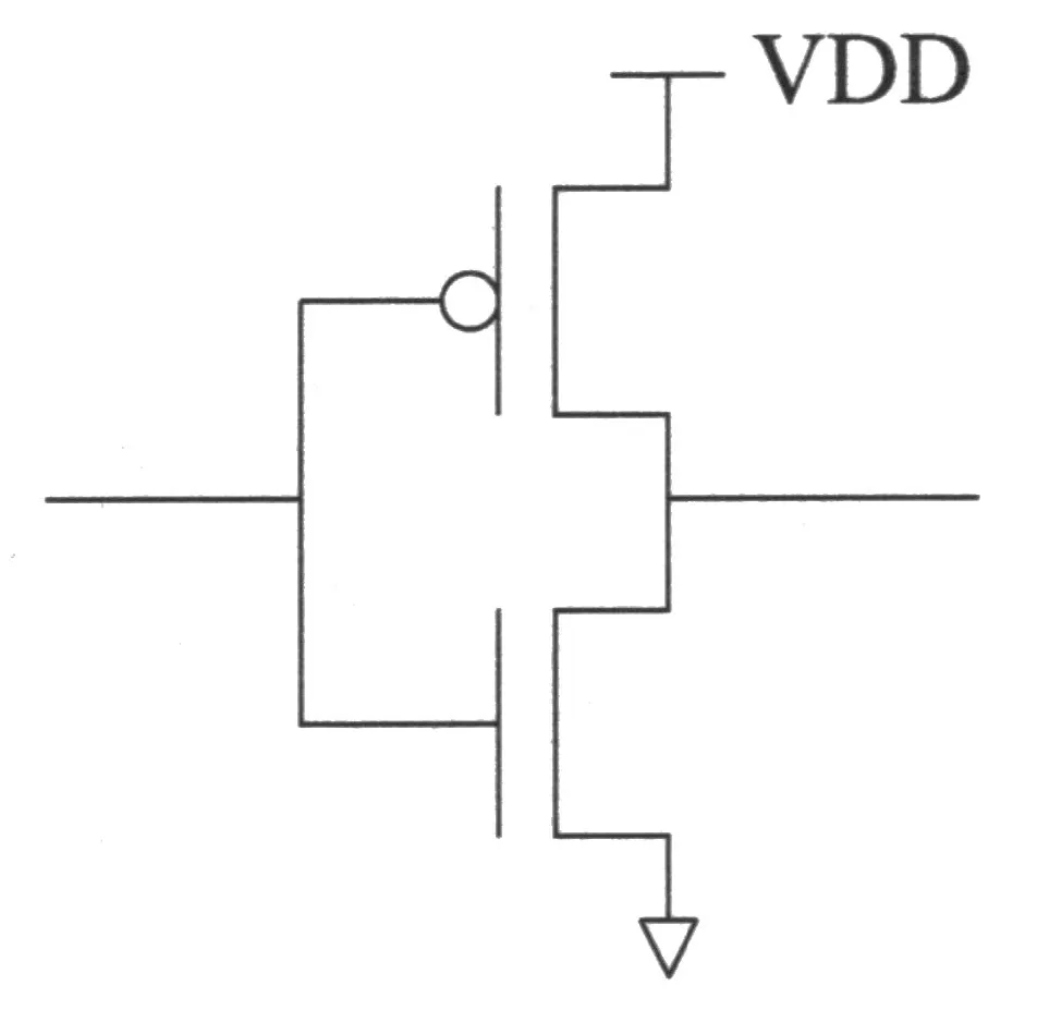
The question (FN10-2, p3, in the paper’s words). Consider an inverter operating with a supply voltage of $V_{DD}$ with logic signals that swing between ground and $V_{DD}$VDD​. (assume $V_T > 0.2$ V; a handwritten addition on the paper.) (a) Let $V_{DD}$ = 0.2 V. Assume that the $I_{off}$ of each transistor is 10 nA. (For the nFET, $I_{off}$ is defined by $V_{GS}$ = 0.0 V and $V_{DS} = V_{DD}$VDD​. For the pFET, $I_{off}$ is defined by $V_{SG}$ = 0.0 V and $V_{SD} = V_{DD}$VDD​.) If the subthreshold slope is 80 mV/decade, what is the $I_{on}/I_{off}$ ratio for each transistor? (For the nFET, $I_{on}$ is defined by $V_{GS} = V_{DD}$ and $V_{DS} = V_{DD}$VDD​. For the pFET, $I_{on}$ is defined by $V_{SG} = V_{DD}$ and $V_{SD} = V_{DD}$VDD​.) (10 points)

FN10-2’s inverter (Final 2010, p3, redrawn), with part (c)‘s operating point added: input $0.9V_{DD}$ (the output of an identical stage), output $0.1V_{DD}$0.1VDD​. The off PFET leaks $I_P = I_{off}10^{0.1V_{DD}/S}$ ($V_{SG} = 0.1V_{DD}$VSG​=0.1VDD​); the on NFET, with only $0.1V_{DD}$ across it, sinks $I_N = I_{off}10^{0.9V_{DD}/S}(1 - e^{-0.1V_{DD}/(kT/q)})$e−0.1VDD​/(kT/q)). At the lowest working supply the two are equal.

The exam’s own figure (FN10-2, p3)

FN10-2, p3 (source figure).

Part (c): the lowest supply for a 10–90 % swing (10 points)

FN10-2c, p4. Imagine that we continue to scale down $V_{DD}$VDD​. Find the lowest value of $V_{DD}$ at which the inverter will operate with an output swing of at least $0.1V_{DD}$ to $0.9V_{DD}$0.9VDD​. What is the $I_{on}/I_{off}$ ratio for each transistor at this value of $V_{DD}$VDD​? (10 points)

Hint

With the output low, which device carries current in, which carries it out, and what are each one’s gate and drain voltages if the input comes from an identical inverter?

What it asks. A supply voltage: the lowest at which the low output still reaches $0.1V_{DD}$ (and, by symmetry, the high output $0.9V_{DD}$0.9VDD​). Then part (a)‘s ratio, $I_{on}/I_{off}$ “for each transistor”, at that supply. “Continue to scale down” says the devices stay subthreshold; “output swing of at least” sets the criterion.

The idea. With the output low, the “on” NFET pulls down while the “off” PFET leaks current in, and at the steady level the two are equal. Below threshold the NFET wins by only about $10^{V_{DD}/S}$10VDD​/S, so the low output rises as $V_{DD}$ falls; it settles where the NFET’s drain factor, small because its $V_{DS}$ is only the low output, cuts its current to the PFET’s leakage. Set $V_{out} = 0.1V_{DD}$0.1VDD​, with the input from an identical stage at $0.9V_{DD}$0.9VDD​, and find the $V_{DD}$ that balances the currents.

Why this formula. $10^{-0.8V_{DD}/S} = 1 - e^{-0.1V_{DD}/(kT/q)}$e−0.1VDD​/(kT/q), and $I_{on}/I_{off} = 10^{V_{DD}/S}$10VDD​/S.

• Where it comes from. NFET: $V_{GS} = 0.9V_{DD}$0.9VDD​, $V_{DS} = 0.1V_{DD}$0.1VDD​: $I_N = I_{off}10^{0.9V_{DD}/S}(1 - e^{-0.1V_{DD}/(kT/q)})$e−0.1VDD​/(kT/q)). PFET: $V_{SG} = 0.1V_{DD}$0.1VDD​, $V_{SD} = 0.9V_{DD}$0.9VDD​, whose drain factor is close to 1: $I_P = I_{off}10^{0.1V_{DD}/S}$Ioff​100.1VDD​/S. Equal currents; divide by $I_{off}10^{0.9V_{DD}/S}$Ioff​100.9VDD​/S.
• Why the drain factor. Without it the NFET’s current would not depend on its drain voltage, so the currents could not balance at any output level: the drain-independent model cannot set an output level at all.
• Conditions. Equal $I_{off}$ and $S$ for both devices (the paper’s), so the high output is the mirror image of the low one and one condition gives both. $kT/q$ = 26 mV (room temperature, added). The paper’s “logic signals that swing between ground and $V_{DD}$VDD​” could be read as a full-rail input instead; that reading gives a lower supply (below), so say which you use.
• The ratio. Part (a) defines $I_{on}/I_{off}$ for each transistor at $V_{GS} = V_{DD}$ against 0, both with $V_{DS} = V_{DD}$VDD​: $10^{V_{DD}/S}$10VDD​/S. It is not the ratio of the NFET’s and PFET’s currents at the operating point.

FN10-2c

1. The currents at the low output. Because the input is $0.9V_{DD}$ and the output $0.1V_{DD}$0.1VDD​: $I_N = I_{off}10^{0.9V_{DD}/S}(1 - e^{-0.1V_{DD}/(kT/q)})$ (its $V_{DS}$ is only $0.1V_{DD}$0.1VDD​, so its drain factor is small); $I_P = I_{off}10^{0.1V_{DD}/S}$ (its $V_{SD} = 0.9V_{DD}$0.9VDD​, factor ≈ 1).
2. Balance. Because the output draws no other current, $I_N = I_P$IP​; $I_{off}$ cancels: $10^{-0.8V_{DD}/S} = 1 - e^{-0.1V_{DD}/(kT/q)}$e−0.1VDD​/(kT/q), that is, with $S$ = 0.08 V and $kT/q$ = 0.026 V, $10^{-10V_{DD}} = 1 - e^{-3.85V_{DD}}$e−3.85VDD​.
3. Solve. Because the left side falls and the right side rises with $V_{DD}$VDD​, there is one crossing; by successive approximation $V_{DD}$ = 65.3 mV. At it both sides equal 0.222: the NFET’s gate drive, $10^{0.8V_{DD}/S}$ = 4.50 times the PFET’s, is cut by its drain factor to exactly the PFET’s leakage.
4. The ratio. Because $I_{on}/I_{off} = 10^{V_{DD}/S}$ for each device (part (a)‘s definition): $10^{65.3/80}$ = 6.56 (6.49 at a rounded 65 mV). The same for the NFET and the PFET.
5. The other readings. Because the PFET’s own drain factor, $1 - e^{-0.9V_{DD}/(kT/q)}$e−0.9VDD​/(kT/q), is about 0.9 at this supply, keeping it lowers the answer to 62.0 mV; with a full-rail input (NFET at $V_{GS} = V_{DD}$VDD​, PFET at $V_{SG} = 0$0) the limit is 52.8 mV (both drain factors kept). The self-consistent reading with the NFET’s factor (65.3 mV) is the one a chain of identical gates needs.

Part (c)‘s balance (computed with $S$ = 80 mV/decade and $kT/q$ = 26 mV). Left of the crossing the dashed side is below the solid one: the NFET, with only $0.1V_{DD}$ across it, cannot sink the PFET’s leak, and the output stays above $0.1V_{DD}$0.1VDD​. The crossing is the lowest working supply, $V_{fn}$ = 65.3 mV, where both sides are 0.222.

Check. By the output level on either side of the answer (both drain factors kept, solving the balance for $V_{out}$Vout​): at 100 mV the low output is 2.7 mV, $0.027V_{DD}$0.027VDD​, comfortably valid; at 50 mV it is $0.153V_{DD}$0.153VDD​, invalid. The 10 % crossing lies between, as found. By size: an ideal 60 mV/decade device would do better; at 80 mV/decade the limit is a little under one decade of gate voltage, where the on/off ratio is only about 6.5.

Answer: $V_{DD} \approx$ 65 mV (65.3 mV: $10^{-0.8V_{DD}/S} = 1 - e^{-0.1V_{DD}/(kT/q)}$e−0.1VDD​/(kT/q), with the input from an identical stage at $0.9V_{DD}$ and the NFET’s drain factor). There, $I_{on}/I_{off} = 10^{V_{DD}/S} \approx$ 6.5 for each transistor (6.56; 6.49 at 65 mV).

Remember. The functional limit comes from the drain factor: the on device’s current falls as its $V_{DS}$ falls, until it only matches the off device’s leakage. Balance the two currents at the output level you need. $I_{on}/I_{off}$ is always $10^{V_{DD}/S}$10VDD​/S.

The key’s working (FN10-2c, p4, the key’s handwriting)

FN10-2c’s key (p4): the same balance and 65 mV; its last line takes "$I_{on}/I_{off}$" as $10^{0.8V_{DD}/0.08} = 4.47$ (see the verdict).

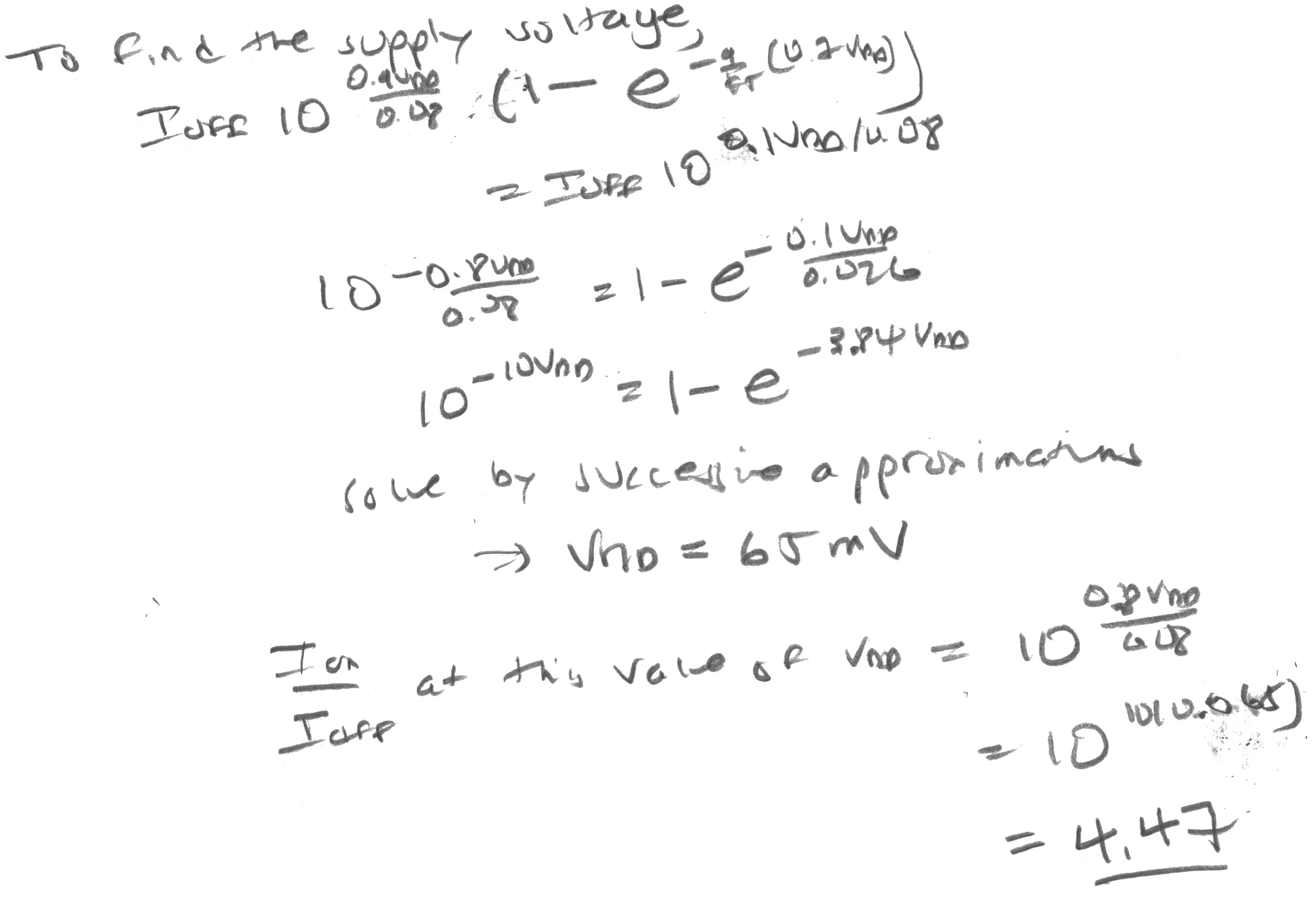
The answer key differs

The key’s supply agrees: the same balance, $10^{-10V_{DD}} = 1 - e^{-3.84V_{DD}}$e−3.84VDD​, solved to 65 mV. Its on/off ratio does not: it writes $I_{on}/I_{off} = 10^{0.8V_{DD}/0.08} = 10^{10(0.065)} = 4.47$4.47, which is the ratio of the NFET’s drive at $V_{GS} = 0.9V_{DD}$ to the PFET’s at $0.1V_{DD}$0.1VDD​, not part (a)‘s ratio. By part (a)‘s definition ($V_{GS} = V_{DD}$VGS​= against 0) the ratio is $10^{V_{DD}/S} = 10^{0.065/0.08} = 6.49$ (6.56 at 65.3 mV).

FN17-10c: the supply for minimum energy (about 8 points)

You need

FN17-10a–b, solved on FN2. Each inverter’s input is $(10 + 5)$ µm × 2 fF/µm = 30 fF, so every node of the chain carries $C$ = 30 fF (the last one the 30 fF load). (a) $I_{on} = 10\ \text{nA}\cdot 10^{V_{DD}/0.08}$10VDD​/0.08. (b) Each stage’s 50 % delay is $CV_{DD}/(2I_{on})$CVDD​/(2Ion​); the chain’s is $8 \times 30\ \text{fF}\cdot V_{DD}/(2I_{on}) = 12\ \mu\text{s/V}\cdot V_{DD}\cdot 10^{-V_{DD}/0.08}$10−VDD​/0.08, 7.59 ns at 0.2 V (the key times the full swing, $CV_{DD}/I_{on}$CVDD​/Ion​: 15.2 ns).

Switching and leakage energy (Chapter 6 §6). A node that rises draws $CV_{DD}^2$ from the supply (half stored, half lost); one that falls draws nothing. A static gate with $V_{DD}$ across its off device dissipates $V_{DD}I_{off}$VDD​Ioff​, so over a time $T$ it uses $V_{DD}I_{off}T$VDD​Ioff​T.

The functional limit (FN10-2c above). With $S$ = 80 mV/decade and $kT/q$ = 26 mV, an inverter driven by its twin gives a 10–90 % swing only down to about 65 mV.

The question (FN17-10, p21–22, in the paper’s words). Consider a chain of eight identical $10\,\mu m/5\,\mu m$ inverters. The chain is loaded at the end by 30 fF. In this problem, we are going to calculate the supply voltage at which this inverter chain will consume minimum energy. This will be subthreshold operation. Let the gate capacitance per unit width be given by 2 fF/µm. (a) Assume the $I_{off}$ of each transistor is 10 nA. If the subthreshold slope is 80 mV/decade, what is the on-current of the devices of the inverter as a function of $V_{DD}$VDD​? (b) Estimate the delay of the inverter chain (as a function of $V_{DD}$VDD​). (The point values are overwritten on the scan; each appears to be 8.)

The chain’s energy model (Chapter 23 §16, added). For FN17-10, $N = N_g = 8$ inverters of $10/5$ µm, every node $C$ = 30 fF (the last one the 30 fF load), $I_{off}$ = 10 nA, $S$ = 80 mV/decade. The transition’s time $T = Nt_p$ is set by the stages charging with $I_{on}$ one after another; meanwhile every inverter leaks $I_{off}$ through its off device. The paper prints no figure for this question.

Part (c): the switching energy and the supply that minimizes it (about 8 points)

FN17-10c, p22. Estimate the switching energy of the inverter chain as a function of $V_{DD}$VDD​. Include both the dynamic power dissipated and the leakage of all the inverters during the delay time of the chain. What value of $V_{DD}$ minimizes this energy? (Point value overwritten on the scan; it appears to be 8.)

Hint

Write the dynamic energy and the leakage energy each as something times $CV_{DD}^2$CVDD2​. As $V_{DD}$ falls, which factor shrinks and which grows, and which wins?

What it asks. $E(V_{DD})$ for one transition through the chain, made of two terms the paper names: the switching energy and the leakage energy of all eight inverters over the chain’s delay. Then the supply at its minimum. “This will be subthreshold operation” keeps the whole calculation below $V_T$VT​.

The idea. Lowering the supply saves switching energy as $V^2$V2, but slows every stage tenfold for each 80 mV, so the eight inverters leak for longer. Both terms carry $CV^2$CV2; the leakage factor grows as $V$ falls, but in this chain never fast enough to beat the $V^2$V2. The energy falls all the way down, so it is lowest at the lowest supply that still works: FN10-2c’s functional limit.

Why this formula. $E = 4CV^2 + 8\,I_{off}\,V\,T$ with $T = 8\,CV/(2I_{on})$8CV/(2Ion​), so $E = 4CV^2[1 + 8\cdot10^{-V/S}]$10−V/S]; $dE/dV = 0 \Leftrightarrow e^u = 4(u - 2)$2), $u = V\ln 10/S$Vln10/S.

• Where it comes from. Switching: in one transition through eight inverters, alternate nodes rise; 4 rising nodes of $C$ = 30 fF draw $4CV^2$4CV2. Leakage: each inverter has one off device with $V$ across it, leaking $I_{off}$Ioff​, for the chain’s delay $T$T: $8I_{off}VT = 8I_{off}V\cdot 4CV/(I_{off}10^{V/S}) = 32CV^2\,10^{-V/S}$32CV210−V/S. $I_{off}$ cancels.
• The stationary point. With $E \propto u^2(1 + 8e^{-u})$8e−u): $dE/du = 2u\,e^{-u}(e^u - 4u + 8)$8). The bracket’s smallest value, at $u = \ln 4 = 1.386$1.386, is $4 - 4\ln 4 + 8 = 6.45 > 0$0. So $dE/dV > 0$ for every $V > 0$0: no minimum. In the general form, $K = N/(4\alpha) = 8/(4 \times \tfrac12) = 4$4, below $e^3 = 20.1$20.1.
• Conditions. The course’s 50 % delay. With the key’s full-swing delay $CV/I_{on}$ the leakage term doubles, $E = 4CV^2[1 + 16\cdot 10^{-V/S}]$10−V/S], the condition becomes $e^u = 8(u - 2)$2), and its bracket’s minimum (at $u = \ln 8$ln8) is 7.36: still no root. DIBL ignored; the model holds only above the functional limit.
• The tempting alternative. Writing the switching term as $4CV$ and the leakage as $I \cdot T$ (both charges, not energies) and minimizing that: it has a minimum, at 132 mV, but of the charge drawn from the supply, not of the energy (the KeyNote).

FN17-10c

1. The switching energy. Because four of the eight nodes rise in one transition, each drawing $CV^2$CV2: $E_{dyn} = 4CV^2 = 4 \times 30\ \text{fF}\times V^2$V2.
2. The leakage energy. Because all eight inverters leak $I_{off}$ with $V$ across them for the chain’s delay $T = 8CV/(2I_{on})$8CV/(2Ion​): $E_{leak} = 8I_{off}VT = 32CV^2\cdot10^{-V/0.08}$10−V/0.08. $I_{off}$ cancels; only $I_{off}/I_{on} = 10^{-V/S}$ remains.
3. The total. $E = 4CV^2\big[1 + 8\cdot10^{-V/0.08}\big]$10−V/0.08]. The bracket grows as $V$ falls (leakage per operation), the $V^2$ shrinks.
4. Look for a stationary point. Because $u = V\ln 10/S$ turns $10^{-V/S}$ into $e^{-u}$e−u, $E \propto u^2(1 + 8e^{-u})$ and $dE/du = 2ue^{-u}(e^u - 4u + 8)$8). Its bracket is smallest where $e^u = 4$4, $u = 1.386$1.386, and is 6.45 there: always positive. $E$ rises with $V$ everywhere; there is no interior minimum.
5. So go as low as the chain works. Because the energy keeps falling as $V_{DD}$ falls, the lowest-energy supply is the lowest at which the logic still gives valid levels: FN10-2c’s criterion with the same $S$ = 80 mV/decade and $kT/q$ = 26 mV, $V_{DD} \approx$ 65 mV (65.3). There $E = 1.14$ fJ per transition, against 1.74 fJ at 100 mV and 4.92 fJ at 200 mV.
6. When would a minimum exist? Because in general $e^u = K(u - 2)$ with $K = N/(4\alpha)$ has a root only for $K \ge e^3 \approx 20.1$20.1, a minimum-energy supply above the functional limit needs deep, quiet logic, $N/\alpha \ge 80$80: many gates leaking for every one that switches. This chain has $K = 4$4.

When a minimum-energy supply exists (Chapter 23 §16): FN17-10’s chain is the dashed $K = 4$ line, which never meets $e^u$eu. Original figure ↗

FN17-10c’s energy per transition (computed from $E = 4CV^2[1 + 8\cdot10^{-V/S}]$ with $C$ = 30 fF; dashed $E_{dyn}$Edyn​, dotted $E_{leak}$Eleak​). $E$ rises for every $V_{DD}$VDD​: there is no minimum, and the energy is lowest at the functional limit, $V_{fn}$ = 65.3 mV, 1.14 fJ (shaded below it: the inverters no longer work). The open circle is the root of the key’s charge form, 132.1 mV (the key’s iteration stops at 0.133 V); it minimizes a charge, not this energy, and the energy there is 2.47 fJ.

Check. By numbers: $E$ = 1.14, 1.74, 2.47, 4.92 and 10.82 fJ at 65.3, 100, 132.1, 200 and 300 mV, rising throughout, as step 4 says. By the leakage share: at 65.3 mV, $E_{leak}/E_{dyn} = 8 \times 10^{-65.3/80} = 1.22$1.22, so leakage is 55 % of the total; it grows as $V$ falls, but the $V^2$ falls faster. By the limit’s role: the model’s $E \to 0$ as $V \to 0$ only because it ignores that the logic stops working; the functional limit is where the model must stop.

Answer: $E(V_{DD}) = 4CV_{DD}^2 + 8\,I_{off}V_{DD}T = 4(30\ \text{fF})V_{DD}^2\big[1 + 8\cdot10^{-V_{DD}/0.08}\big]$ (with the course’s 50 % delay $T = 8CV_{DD}/(2I_{on})$8CVDD​/(2Ion​); $16$ in place of 8 with the full-swing delay). $dE/dV_{DD}$ is positive for every $V_{DD}$VDD​: there is no interior minimum. The energy keeps falling as $V_{DD}$ falls, so the minimum-energy supply is the lowest working supply, about 65 mV by FN10-2c’s 10–90 % criterion, where $E \approx 1.1$ fJ per transition. (The key’s 0.133 V minimizes the charge drawn, not the energy.)

Remember. Energy is $CV^2$CV2, and leakage energy is $I_{off}V$ times the operation’s time. Test $K = N/(4\alpha)$ against $e^3 \approx 20$20: below it, there is no minimum-energy supply, and the answer is the functional limit. On the exam, write the energy with $V^2$V2, state the result, and say that the intended 0.133 V is the charge form’s answer.

The key’s working (FN17-10c, p22, the key’s handwriting)

FN17-10c’s key (p22): both terms are written without a factor $V_{DD}$VDD​, $4(30\ \text{fF})V_{DD}$ and the delay times $8 \times 10$ nA, so the expression it minimizes is a charge (see the verdict).

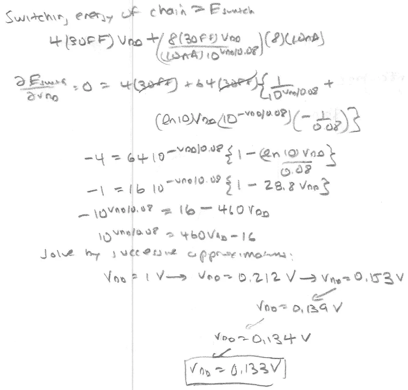
The answer key differs

The key writes the “switching energy” as $4(30\ \text{fF})V_{DD} + \text{delay} \times 8 \times 10\ \text{nA}$ (with the full-swing delay $8(30\ \text{fF})V_{DD}/I_{on}$8(30 fF)VDD​/Ion​): both terms are charges (C·V and I·t), each missing a factor $V_{DD}$VDD​; the transcription’s own note flags the first. Minimizing that charge gives $10^{V_{DD}/0.08} = 460V_{DD} - 16$ and, by its iteration, 0.133 V (the root is 132.1 mV). The energy the part asks for, $4CV_{DD}^2[1 + 16\cdot 10^{-V_{DD}/0.08}]$ in the key’s delay convention, has $dE/dV_{DD} > 0$ everywhere ($e^u = 8(u - 2)$eu= has no root; $e^u - 8u + 16 \ge 7.36$7.36), so it has no minimum above the functional limit. At 132.1 mV the energy (with the course’s 50 % delay) is 2.47 fJ, 2.17 times its value at 65.3 mV; in the key’s full-swing form it is 1.61 times.

Harder variations: the lowest supply and minimum energy

You need

The functional limit (FN10-2c). Balance $I_{off}10^{0.9V/S}(1 - e^{-0.1V/(kT/q)}) = I_{off}10^{0.1V/S}$ and solve for $V$V; with $S$ and $kT/q$ both scaled by a factor, the solution scales by the same factor.

Energy per operation (FN17-10c). $E = N_gCV^2[\alpha + (N/2)10^{-V/S}]$(N/2)10−V/S]; a stationary point needs $e^u = K(u - 2)$2), $u = V\ln 10/S$Vln10/S, $K = N/(4\alpha) \ge e^3 \approx 20.1$20.1. With two roots, the larger ($u > 3$u>3) is a local minimum, to be compared with the energy at the functional limit; iterate $u \leftarrow \ln K + \ln(u - 2)$ from $u = 6$6. At the minimum, $E_{leak}/E_{dyn} = 2/(u - 2)$2).

Subthreshold delay (FN17-10b). The chain’s 50 % delay is $N\,CV/(2I_{off}10^{V/S})$NCV/(2Ioff​10V/S).

FN10-2’s inverter (p3). Original figure ↑

These variations added push the two past parts into setups no paper uses: Variation 6 is a block where the minimum-energy supply does exist, found and checked against the functional limit; Variation 7 moves FN17-10’s chain to a hot corner and adds a speed requirement, so the answer is set by whichever limit binds. No key exists, so there is no key verdict.

Variation 6: a deep, quiet block where the minimum exists (about 25 minutes)

Variation 6: a deep, quiet block where the minimum exists

added The question. A sensor’s signal-processing block has $N_g$ = 2,000 gates, each driving $C$ = 4 fF; its critical path is $N$ = 60 gates deep; per operation only $\alpha$ = 0.08 of the nodes rise. The devices have $S$ = 85 mV/decade (for example), $kT/q$ = 26 mV, and the block runs subthreshold ($V_T$VT​ = 0.35 V). (a) Does a minimum-energy supply exist? (b) Find it. (c) Compare its energy per operation with the energy at the functional limit and at 0.3 V. (d) What share of the energy is leakage at the minimum? (e) If the activity doubles to $\alpha$ = 0.16, which way does the minimum move?

Variation 6’s energy per operation (computed from $E/(N_gC) = V^2[\alpha + 30\cdot10^{-V/S}]$ with $S$ = 85 mV/decade). With $K = 187.5 > e^3$ the curve has a true minimum: 251.1 mV and $7.15 \times 10^{-3}$ V² for $\alpha$ = 0.08 (solid), far below its 22.35 at the functional limit $V_{fn}$ = 67.9 mV. Doubling the activity to 0.16 (dashed) moves the minimum down to 217.9 mV.

Hint

Compute N/(4α) first. Which root of the stationary condition is the minimum?

What it asks. The full minimum-energy calculation where the answer is an interior point: the existence test, the root, and the checks that it is a minimum, above the functional limit and below threshold.

The idea. With deep, low-activity logic, many gates leak for every one that switches, so leakage per operation grows fast as the supply falls and the slower operation lengthens it: below some supply the leakage term wins and the energy turns up again. The existence test says when; the iteration finds where.

Why this formula. $E/(N_gC) = V^2[\alpha + (N/2)10^{-V/S}]$ and $e^u = K(u - 2)$ (approach 3).

• Where it comes from. $dE/dV = 0$0: $2\alpha + N e^{-u} = (N/2)ue^{-u}$(N/2)ue−u, so $e^u = (N/(4\alpha))(u - 2)$2).
• Conditions. The larger root ($u > 3$u>3) is a local minimum (the smaller is a maximum), so it must also beat the energy at the functional limit, step 3; the iteration $u \leftarrow \ln K + \ln(u - 2)$ converges to it from $u = 6$6.

Variation 6

1. (a) Existence. Because $K = N/(4\alpha) = 60/(4 \times 0.08) = 187.5 \ge e^3 = 20.1$20.1: yes.
2. (b) The root. Because the iteration $u \leftarrow \ln 187.5 + \ln(u - 2)$ from 6 settles at $u = 6.803$6.803: $V_{min} = uS/\ln 10 = 6.803 \times 0.085/2.303 = 251.1$ mV, below $V_T$ (subthreshold holds). The other root, $u = 2.041$2.041, is a maximum.
3. (c) Against the limits. Because the functional limit at 85 mV/decade is 67.9 mV, $V_{min}$ is far above it. $E/(N_gC)$E/(Ng​C): $7.15 \times 10^{-3}$ V² at 251.1 mV, $22.35 \times 10^{-3}$ at 67.9 mV, $8.00 \times 10^{-3}$ at 0.3 V. With $N_gC = 2000 \times 4$ fF = 8 pF: 57.2 fJ per operation at the minimum against 178.8 fJ at the functional limit.
4. (d) Leakage share. Because at the minimum $E_{leak}/E_{dyn} = 2/(u - 2) = 0.416$0.416, leakage is $2/u = 29.4$ % of the total.
5. (e) More activity. Because $K = 60/(4 \times 0.16) = 93.75$93.75, the root falls to $u = 5.902$5.902, $V_{min}$ = 217.9 mV: down. More switching per operation makes leakage relatively cheaper, so the optimum moves toward lower supply.

Check. By the stationary condition itself: at $u = 6.803$6.803, $e^u$ and $K(u - 2) = 187.5 \times 4.803$ both come to 900.6. By the energy on either side: 8.00 at 0.3 V and far more at 67.9 mV, both above 7.15 at 251 mV.

Answer: (a) yes, $K = 187.5 \ge 20.1$20.1. (b) $V_{min}$ = 251 mV ($u = 6.803$u=6.803). (c) 57.2 fJ per operation, against 178.8 fJ at the 67.9 mV functional limit (and $8.00 \times 10^{-3} \times 8$ pF = 64.0 fJ at 0.3 V). (d) 29.4 % leakage. (e) down, to 218 mV.

Remember. Deep and quiet ($N/\alpha \ge 80$N/α≥80) logic can have a minimum-energy supply, at a few $S/\ln 10$S/ln10, once its energy also beats the functional limit’s, as (c) checks; at it leakage is $2/u$ of the energy, about a third. More activity moves it lower.

Variation 7: FN17-10’s chain, hot and against a deadline (about 25 minutes)

Variation 7: FN17-10’s chain, hot and against a deadline

added The question. FN17-10’s chain (eight inverters, $C$ = 30 fF per node, $I_{off}$ = 10 nA, $S$ = 80 mV/decade at 300 K, 50 % delays) must finish each transition within 50 ns, and must work from 300 K to 358 K (85 °C). Take $S$ and $kT/q$ to scale with absolute temperature (the ideality fixed), and $I_{off}$ to rise to 100 nA when hot (for example). (a) The hot $S$S, $kT/q$ and functional limit. (b) The lowest cold supply that meets 50 ns, and the cold chain’s delay at the cold functional limit. (c) Is the deadline at risk when hot? (d) Which supply do you choose, and what does a transition cost, cold and hot?

Variation 7’s delays (computed from the chain’s 12 µs/V × $V\cdot10^{-V/S}$10−V/S, scaled by $10\ \text{nA}/I_{off}$10 nA/Ioff​): cold ($S$S = 80 mV/decade, $I_{off}$ = 10 nA, solid) and hot ($S$S = 95.5 mV/decade, $I_{off}$ = 100 nA, dashed). The cold chain meets 50 ns from 115.4 mV up; at its $V_{fn}$ = 65.3 mV it takes 119.6 ns. Hot, the chain is faster (8.56 ns at 115.4 mV), but its functional limit rises to 78.0 mV.

Hint

Which corner is slowest, which corner gives the worst logic levels, and does the energy argument of FN17-10c still say “as low as possible”?

What it asks. The same chain with two more constraints: a speed requirement, which sets a floor on the supply cold, and a temperature range, which moves the functional limit. The chosen supply is the highest of the floors, because FN17-10c showed the energy keeps falling with $V_{DD}$VDD​.

The idea. Heat raises $kT/q$ and with it $S$S, so the subthreshold characteristic stretches: the functional limit moves up in proportion. Heat also raises $I_{off}$Ioff​, which speeds the chain, so speed is a cold problem and levels a hot one. Energy still falls with the supply, so pick the lowest supply that satisfies both.

Why this formula. The functional-limit balance (FN10-2c), the chain’s delay $T = 8CV/(2I_{off}10^{V/S})$8CV/(2Ioff​10V/S), and $E = 4CV^2[1 + 8\cdot 10^{-V/S}]$ (FN17-10c; $I_{off}$ cancels from it).

• Where it comes from. The balance depends on $V$ only through $V/S$ and $V/(kT/q)$V/(kT/q): scale both by $k$ and the solution scales by $k$k.
• Conditions. The ideality factor fixed (so $S \propto T$T); DIBL ignored.

Variation 7

1. (a) Hot. Because $S$ and $kT/q$ scale by $358/300 = 1.193$1.193: $S$ = 95.5 mV/decade, $kT/q$ = 31.0 mV, and the functional limit moves from 65.3 mV to $65.3 \times 1.193 = 78.0$ mV.
2. (b) Cold speed. Because $T = 12\ \mu\text{s/V}\cdot V\cdot10^{-V/0.08} \le 50$ ns: by successive approximation $V \ge$ 115.4 mV. At the cold functional limit, 65.3 mV, the chain would take 119.6 ns, too slow: the deadline, not the levels, sets the cold floor.
3. (c) Hot speed. Because $I_{off}$ is ten times larger and $S$ larger: at 115.4 mV the chain takes 8.56 ns; even at the hot limit, 78.0 mV, 14.3 ns. The delay’s $V\cdot10^{-V/S}$ peaks at $V = S/\ln 10 = 41.5$ mV, where the hot chain would take 18.3 ns, so hot it never misses 50 ns.
4. (d) The choice. Because energy falls with $V_{DD}$ and the floors are 115.4 mV (cold speed) and 78.0 mV (hot levels), choose 115.4 mV. A transition then costs 2.06 fJ cold and 2.39 fJ hot (the larger hot $S$ leaves more leakage per operation), against the 1.14 fJ FN17-10c’s chain could reach at 65.3 mV without the deadline.

Check. By the scaling: $78.0/65.3 = 1.193$1.193, the temperature ratio, as step 1’s argument requires. By the energy’s $I_{off}$-independence: the hot energy differs from the cold only through $S$S, since $I_{off}$ cancels from $E_{leak}$Eleak​; with a larger $S$ the factor $10^{-V/S}$ is larger, so the hot energy is higher, as found.

Answer: (a) $S$ = 95.5 mV/decade, $kT/q$ = 31.0 mV, functional limit 78.0 mV. (b) 115.4 mV; at 65.3 mV the cold chain needs 119.6 ns. (c) no: the hot chain is fast (8.56 ns at 115.4 mV, at most 18.3 ns at any supply). (d) 115.4 mV: 2.06 fJ cold, 2.39 fJ hot per transition.

Remember. Speed binds cold, levels bind hot. With no interior energy minimum, the right supply is the highest of the floors.