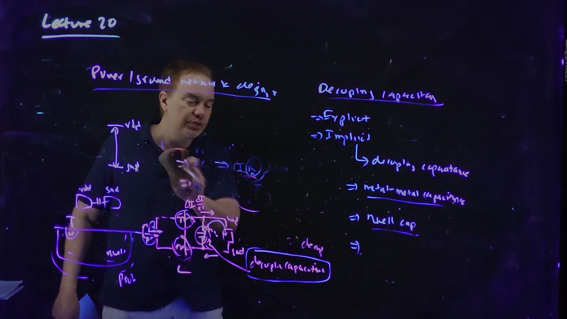
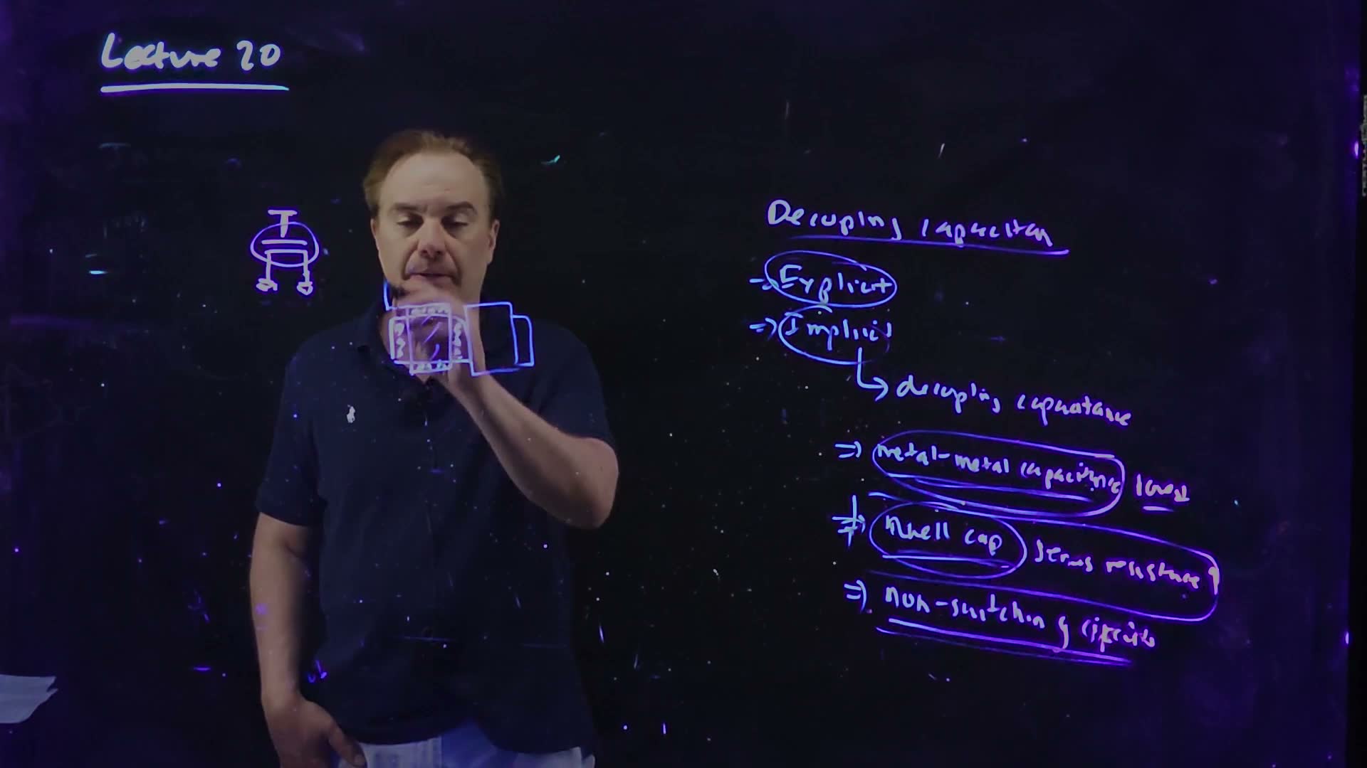
21. Repeaters, crosstalk and supply noise

Chapter 20 left a long wire in trouble: its RC delay grows as the square of its length, while the gates around it keep getting faster. Lecture 20 finishes the story of on-chip wires. It first answers the question Chapter 20 only raised: if you cut the wire into pieces with inverters (repeaters) between them, how many pieces, and how big an inverter? Then it turns to what a wire does to its neighbours. Wires sit side by side, so a switching wire couples a glitch onto a quiet one (enough, at a latch, to flip a stored bit) and changes the delay of one that is switching too. Next comes inductance: when a wire behaves as a transmission line, and why that became possible only once wires got fast. The last third is about the wires that carry power. The supply on chip is never steady; it droops by IR drop and bounces by L dI/dt. Designers fight it with grids on every metal layer and with decoupling capacitance: some of it comes for free, and the rest is built from MOS capacitors tiled into the layout’s white space.

After this chapter you can:

1. write a repeated wire’s delay as $k$ segments of three Elmore terms, and derive the best repeater size $h$ and number $k$k;
2. explain why the best segment length and repeater size do not depend on the wire’s length, and estimate a wire’s delay with and without repeaters;
3. compute the worst coupling glitch from a capacitance divider, explain how it can flip a pass-transistor latch, and list the fixes;
4. give the effective coupling capacitance when the neighbouring wire is quiet, switches the same way, or switches the opposite way;
5. decide from the RC delay, the LC time of flight and the slew time whether a wire’s inductance matters;
6. name the two kinds of supply noise, estimate the delay change a supply droop causes, and give the reasons for power grids;
7. list the sources of on-chip decoupling capacitance, size a decap for an allowed droop, and explain why explicit decap is built from small cells.

Boxes and equations marked board were written in the lecture. Parts marked added are explanations or examples this guide adds.

Symbols

Symbol	Meaning	Unit	First appears
$R$R, $C$	the total resistance and capacitance of the whole wire (the board’s repeater formulas use totals)	Ω, fF	§1
$\mathcal{R}$R, $\mathcal{C}$C, $\mathcal{L}$	resistance, capacitance and inductance per unit length (the board’s script letters)	Ω/µm or Ω/mm, fF/µm or pF/mm, nH/mm	§1, §7
$\ell$	the wire’s length. Chapter 20 and the boards write $L$L; this chapter writes $\ell$ because $L$ is also inductance here	µm, mm	§1
$R_{drv}$Rdrv​, $C_L$	a single driver’s output resistance and the wire’s load (Chapter 20’s form)	Ω, fF	§1
$R_{buf}$Rbuf​, $C_{buf}$	the output resistance and the input capacitance of the minimum inverter	Ω, fF	§1
$R_{buf}C_{buf}$	the minimum inverter driving a copy of itself: its fan-out-of-one delay, the course’s $\tau_{inv}$	ps	§1
$k$	the number of equal segments the wire is cut into: the number of repeaters, counting the original driver	—	§1
$h$	the size of every repeater, in multiples of the minimum inverter: resistance $R_{buf}/h$Rbuf​/h, input $hC_{buf}$	—	§1
$T_{delay}$Tdelay​, $T$	the delay of the whole repeated wire (the board writes $T_{delay}$Tdelay​)	ps	§1
$h_{opt}$hopt​, $k_{opt}$	the best size and the best (continuous) number of segments	—	§2
$T_{min}$	$T$ at the best $h$ and $k$ added	ps	§2
$\ell_{seg}$	the best segment length, $\ell/k$ added	mm	§2
$C_c$	coupling (floating) capacitance: from the victim wire to a wire that switches	fF	§3
$C_g$	ground capacitance: from the victim to everything that does not switch	fF	§3
$\Delta V$	the size of a coupling glitch, or of a supply droop	V	§3, §10
$R_d$	the victim driver’s output resistance added	Ω	§3
$V_{DD}$VDD​, $V_T$VT​, $V_{GS}$	supply voltage, threshold voltage, gate-to-source voltage	V	§3, §4
$m$	the Miller factor: 0, 1 or 2 copies of $C_c$ the victim’s driver feels added	—	§5
$C_{eff}$	the victim’s effective load, $C_g + mC_c$ added	fF	§5
$\Delta t$	how much later a coupled waveform crosses 50%	ps	§5
$L$	the inductance of a current loop	H, nH, pH	§6
$\Phi$	the magnetic flux through the loop	Wb	§6
$\omega$	angular frequency	rad/s	§6
$t_{slew}$	the slew (transition) time of the signals on the wire	ps	§7
$t_{RC}$tRC​, $t_{LC}$	the wire’s RC (Elmore) delay and its LC time of flight	ps	§7
$\ell^{*}$	the length where $t_{RC} = t_{LC}$ added	mm	§7
$\ell_1$	the length where $t_{LC}$ reaches $t_{slew}$	mm	§7
$\ell_{chip}$	the chip’s linear size	mm	§7
$I$	current	A	§6
$S$	supply sensitivity of a delay, $(V_{DD}/\tau)(\partial\tau/\partial V_{DD})$ added	—	§8
$\tau$	a gate (buffer) delay	ps	§8
$\tau_{silicon}$	the gates’ share of a path’s delay (the part that depends on $V_{DD}$VDD​)	ps	§8
$N$	the number of parallel paths in a grid	—	§9
$C_{decap}$	decoupling capacitance between $V_{DD}$ and ground	nF	§10
$C_{sw}$	the load that switches in one edge, taking its charge from the decap added	nF	§10
$\varepsilon$	the allowed droop as a fraction of $V_{DD}$ added	—	§10
$R_s$	the resistance in series with a decap	Ω	§11
$C_{gate}$	a quiet gate’s input capacitance, acting as decap (not $C_g$Cg​)	fF	§11
$C_{ox}$	gate-oxide capacitance per unit area	fF/µm²	§12
$W$W, $L$ (of a cell)	the width and channel length of a MOS decap cell; this $L$ is a length, said where used	µm	§12

1. Repeaters: the delay of a cut-up wire

You need

A driven RC wire (Chapter 20, Lecture 19). A driver of output resistance $R_{drv}$ drives a uniform wire of total resistance $R$ and total capacitance $C$C, spread evenly along it, into a load $C_L$CL​. Its Elmore delay is

$$T = R_{drv}(C + C_L) + \tfrac12 RC + RC_L .$$

The ½ is there because the wire’s charge is spread along it: on average it passes through half the wire’s resistance. $\tfrac12RC$ is the intrinsic delay (the wire against its own capacitance) and $RC_L$ the extrinsic delay (the wire against the load). With $R = \mathcal{R}\ell$ and $C = \mathcal{C}\ell$ the intrinsic term is $\tfrac12\mathcal{R}\mathcal{C}\ell^2$21​RCℓ2: twice the length, four times the delay. Here $\ell$ is Chapter 20’s $L$L, the wire’s length.

The uniform line (Chapter 20, Lecture19 @ 27:59): each slice $\mathcal{C}\,dx$ is charged through the resistance $\mathcal{R}x$ back to the driver. Summing gives $\tfrac12\mathcal{R}\mathcal{C}L^2 + \mathcal{R}LC_{load}$RLCload​; Chapter 20’s $L$ is this chapter’s $\ell$ℓ. Original figure ↗

Resistive shielding (Chapter 20). The wire’s resistance partly hides its far capacitance from the driver, so the lumped term $R_{drv}(C + C_L)$CL​), which makes the driver charge everything at once, overestimates a little.

An inverter as a switch and a resistor (Chapter 7). An inverter $h$ times the minimum size has $h$ times the width, so its output resistance is $R_{buf}/h$ and its input capacitance $hC_{buf}$hCbuf​. The minimum inverter driving a copy of itself takes $R_{buf}C_{buf}$Rbuf​Cbuf​: its fan-out-of-one (FO1) delay, the course’s $\tau_{inv}$τinv​.

The question. A long wire is slow because its delay grows as its length squared. If we cut it into shorter pieces and put an inverter at the start of each piece, every piece is short and fast, but every inverter costs a gate delay. How do we write the delay of the cut-up wire, so that we can then choose the number of pieces and the size of the inverters?

Why cutting helps

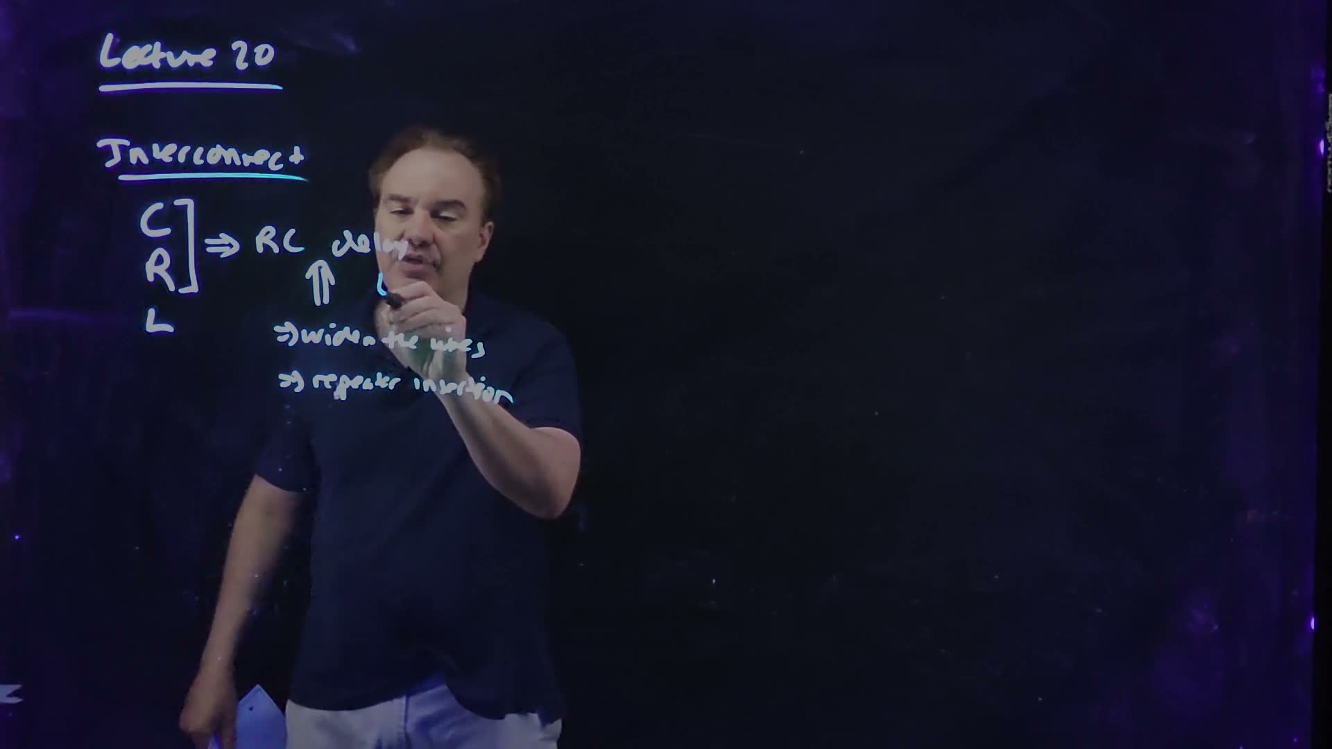
The lecture opens with the recap on the board at 01:37 board: wires have capacitance, resistance and (we shall see) inductance; C and R together give the RC delay; and the RC delay has two fixes, widen the wires (Chapter 20) and repeater insertion. The reason repeaters help is the square law. Cut a wire into $k$ equal pieces: each piece has $1/k$ of the length, so its intrinsic delay is $1/k^2$ of the whole wire’s, and $k$ pieces together take $k \times 1/k^2 = 1/k$ of it. The wire’s own delay falls as $1/k$1/k. What we pay is one inverter per piece (01:32–02:01). Somewhere between “no repeaters” and “a repeater every few microns” is a best choice, and the lecture finds it with a “back of the envelope” model (02:01).

The model: k segments, repeaters of size h

The board’s parameters (02:00–05:29) board:

• $R$R, $C$C: the total resistance and capacitance of the wire.
• $R_{buf}$Rbuf​, $C_{buf}$Cbuf​: the resistance and the input capacitance of the minimum inverter. Its FO1 delay is $R_{buf}C_{buf}$ (“FO1 of minimum sized inverter = $R_{buf}C_{buf}$Rbuf​Cbuf​”).
• One assumption: the repeaters cut the wire into segments of equal length. Unequal segments could do a little better, just as tapering a wire does a little better than widening it uniformly; equal segments get most of the benefit and keep the algebra simple (03:35–04:25).
• $k$k: the number of segments. Each segment has its own driver, so $k$ is also the number of repeaters, counting the original driver.
• $h$h: the size of every repeater, as a multiple of the minimum inverter ($h = 2$h= is twice the minimum, 04:57).

The repeated wire added, drawn for $k = 4$4. The wire of length $\ell$ℓ, total $R$ and $C$C, is cut into $k$ equal segments of $R/k$ and $C/k$C/k. Every segment is driven by an inverter $h$ times the minimum, the first one being the original driver, and the last segment drives a receiver of the same size, whose input is $hC_{buf}$hCbuf​. Because the segments are identical, the whole delay is $k$ times one segment’s.

Every segment is the same circuit (06:07–06:33), so the whole delay is $k$ times one segment’s, and we only need to write one segment’s delay.

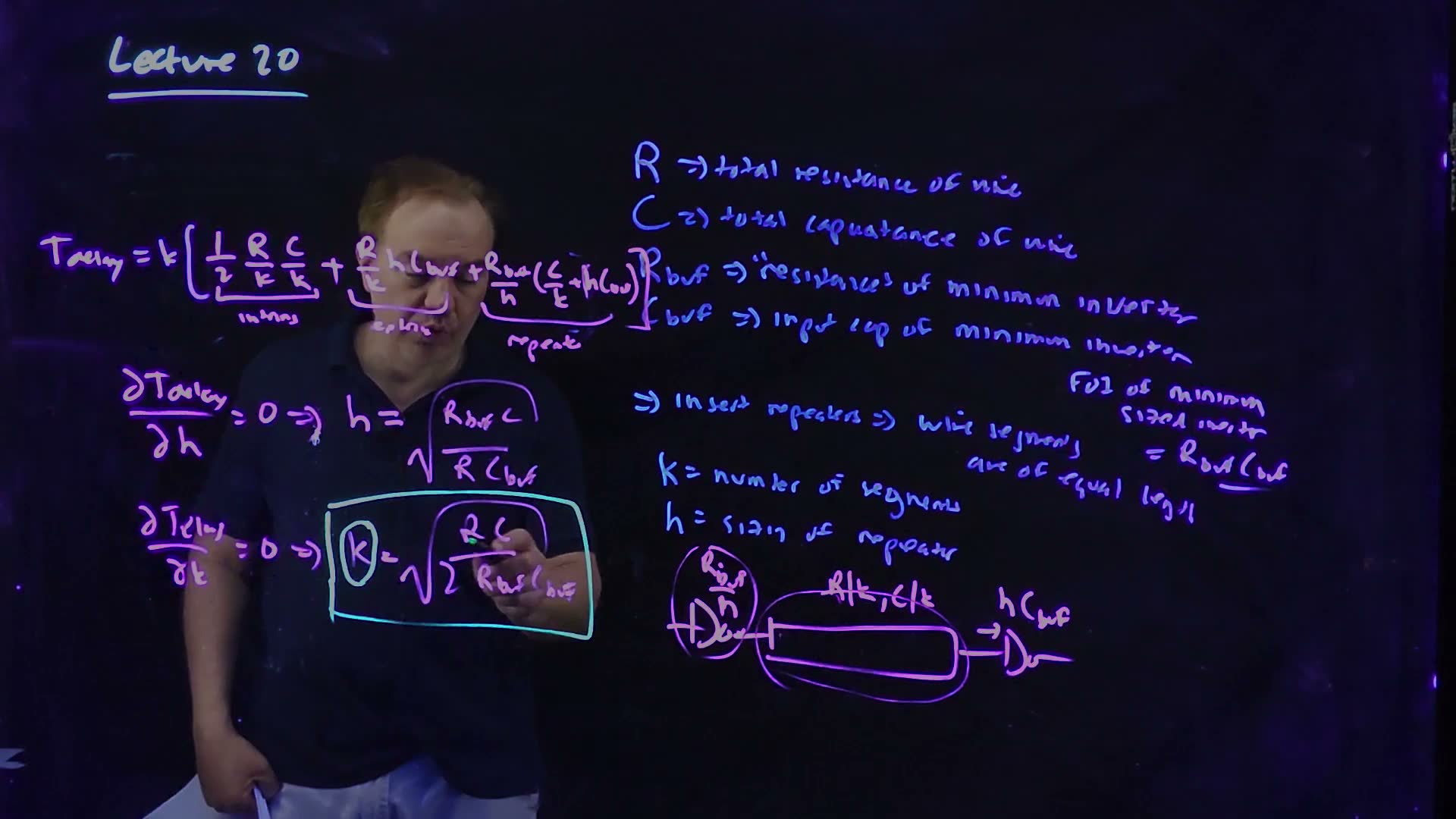
One segment of a repeated wire, redrawn from the board (Lecture20 @ 11:59). A repeater of size $h$ (resistance $R_{buf}/h$Rbuf​/h) drives one $k$-th of the wire ($R/k$R/k, $C/k$C/k) into the next repeater, whose input is $hC_{buf}$hCbuf​. The delay of the whole wire is $k$ times one segment’s Elmore delay, in three terms: the wire’s intrinsic delay (int), the extrinsic delay of the wire’s resistance charging the next repeater (ext), and the repeater’s own resistance charging everything after it (rep).

The board (Lecture20 @ 11:59)

Lecture20 @ 11:59The whole repeater board: the definitions, the segment, the delay with its three braces, and the two optimum results (Section 2).

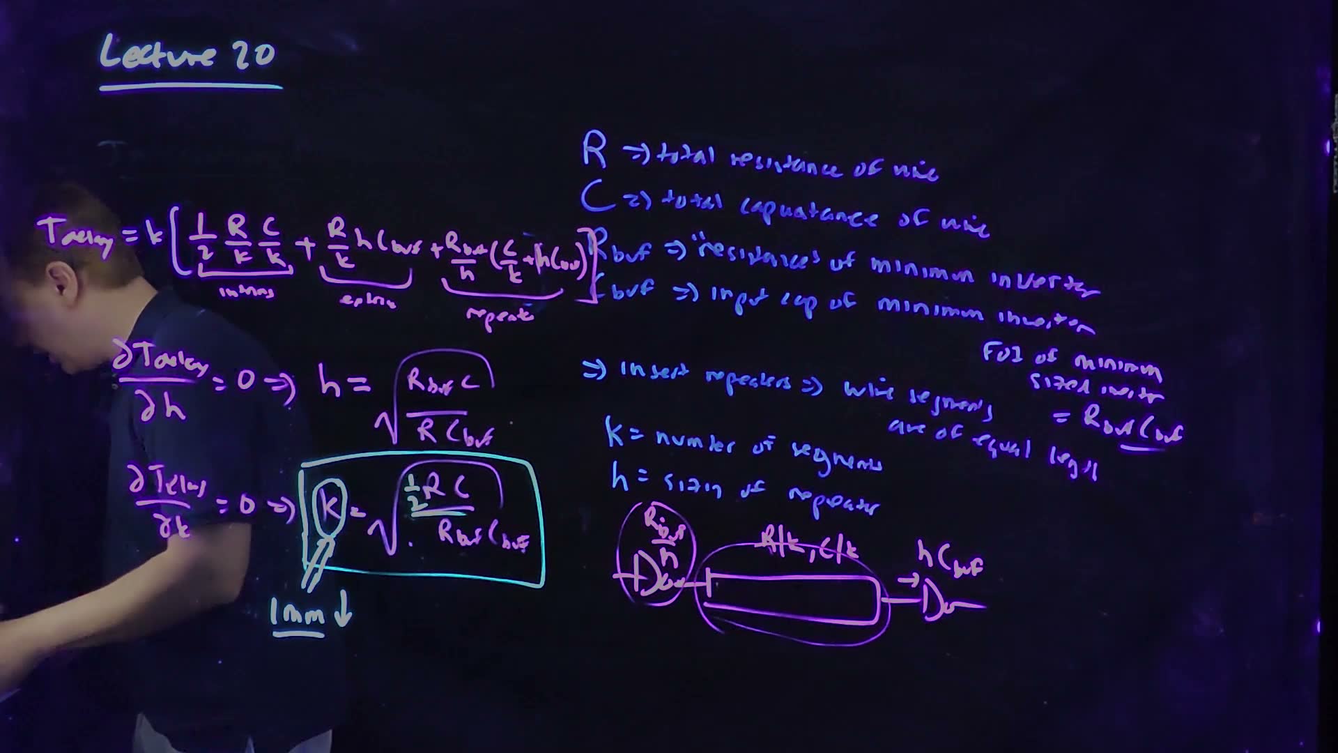
Fair copy of the board above (Lecture20 @ 11:59), mark for mark in its own layout. Teal is the cyan pen, which marks the result: the box round the optimum $k$k, the pointer from it and “1 mm ↓”. Everything else is black: the blue definitions and the violet working and segment drawing. The boxed $k$ first read $\sqrt{RC/(2R_{buf}C_{buf})}$ (09:33); the lecturer then moved the 2 into the numerator as ½, to read it as the intrinsic delay over the FO1 delay. The writing is levelled; the board’s lines drift down to the right.

One segment’s delay: three Elmore terms

Write the segment’s Elmore delay the way Chapter 20 taught: every capacitor times the resistance between it and its driver (06:33–07:39) board. There are two resistances (the repeater’s $R_{buf}/h$ and the wire’s $R/k$R/k) and two capacitances (the wire’s $C/k$C/k, spread along it, and the next input $hC_{buf}$ at its end).

The three terms of one segment’s Elmore delay added, each panel thickening the resistance and the capacitance it pairs. (a) Intrinsic: the wire’s $R/k$ against its own spread $C/k$C/k, with the ½ of a distributed line. (b) Extrinsic: the wire’s $R/k$ against the next repeater’s input $hC_{buf}$hCbuf​. (c) Repeater: the driver’s $R_{buf}/h$ against everything it charges, $C/k + hC_{buf}$hCbuf​, with resistive shielding ignored.

One segment, term by term (board, 06:33–07:39)

1. Intrinsic: the wire against itself. The segment is a distributed wire of $R/k$ and $C/k$C/k, so, as in Chapter 20, its own charge sees half its resistance on average: $\tfrac12\,\dfrac{R}{k}\,\dfrac{C}{k}$21​kR​kC​.
2. Extrinsic: the wire against the next input. The next repeater’s input $hC_{buf}$ sits at the far end, behind all of the segment’s resistance: $\dfrac{R}{k}\,hC_{buf}$kR​hCbuf​.
3. Repeater: the driver against everything. The driving repeater’s resistance $R_{buf}/h$ is in the path of every capacitor in the segment, the wire’s and the next input’s: $\dfrac{R_{buf}}{h}\Big(\dfrac{C}{k} + hC_{buf}\Big)$hCbuf​). This term lets the driver see the whole capacitance at once, which ignores resistive shielding (“I’m of course ignoring resistive shielding here”, 07:39): a small overestimate.
4. All k segments. The segments are identical and in series, so multiply by $k$k.

The delay of a repeated wireboard

$$T_{delay} = k\left[\frac12\,\frac{R}{k}\,\frac{C}{k} + \frac{R}{k}\,hC_{buf} + \frac{R_{buf}}{h}\left(\frac{C}{k} + hC_{buf}\right)\right]$$

Holds when: k equal segments; identical repeaters of size h, each driving its segment and the next repeater's input; Elmore delay; resistive shielding ignored; the repeaters' own output (drain) capacitance not modelled; R and C are the wire's totals

Memorize or derive. Derive it: write one segment’s three Elmore terms (wire against itself with ½, wire against the next input, driver against everything), then multiply by $k$k. Three lines on the exam, and the derivation is what keeps the ½ and the $h$‘s in the right places.

What breaks it. Unequal segments; a last load that is not $hC_{buf}$ (a big receiver, say); long segments with strong repeaters, where resistive shielding is no longer small; a first driver that is given rather than sized $h$ (its own resistance replaces $R_{buf}/h$ in the first segment’s repeater term, and only the $k-1$ inserted repeaters are free to size); and repeaters whose own output capacitance matters (each repeater’s cost in the model is one FO1 delay into the next input, $(R_{buf}/h)\cdot hC_{buf} = R_{buf}C_{buf}$Rbuf​Cbuf​, and nothing for its own drain capacitance).

The same delay as four terms

Multiplying the bracket by $k$ and collecting gives a form that shows what $k$ and $h$ each do added:

$$T = \frac{RC}{2k} + R\,h\,C_{buf} + \frac{R_{buf}C}{h} + k\,R_{buf}C_{buf}.$$

In words, the four terms are: the wire against itself; the wire’s resistance against the repeaters’ inputs; the repeaters’ resistance against the wire; the repeaters against each other’s inputs.

• The wire’s own delay, $RC/(2k)$RC/(2k), falls as $1/k$1/k: the square law at work.
• The repeaters’ delay into each other’s inputs, $kR_{buf}C_{buf}$kRbuf​Cbuf​, rises as $k$k: each repeater adds one FO1 delay.
• The two middle terms do not contain $k$ at all. They depend only on $h$h: a bigger repeater drives the wire faster ($R_{buf}C/h$Rbuf​C/h falls) but loads it more ($RhC_{buf}$RhCbuf​ grows). The wire’s whole resistance meets $h$ inputs’ worth of capacitance in total, and the repeaters’ total drive meets the whole wire, however we cut it.

So $k$ trades the first term against the last, and $h$ trades the two middle ones. Section 2 makes both trades.

A worked example

An added example added: 10 mm of Chapter 20’s example wire, which has 0.076 Ω/□ at 0.4 µm wide, so $\mathcal{R} = 0.19$ Ω/µm, and $\mathcal{C} = 0.1$ fF/µm. Then $R = 1900$ Ω and $C = 1000$ fF $= 1$ pF. Take, for example, a minimum inverter with $R_{buf} = 10$ kΩ and $C_{buf} = 1$ fF, so $R_{buf}C_{buf} = 10$ ps. (1 Ω × 1 fF $= 10^{-3}$ ps.)

10 mm of wire, one minimum inverter

1. The three terms ($k = 1$k=1, $h = 1$1). Intrinsic: $\tfrac12 \times 1900 \times 1000$ fF·Ω $= 950$ ps. Extrinsic: $1900 \times 1$ fF $= 1.9$ ps. Repeater: $10\,000 \times (1000 + 1)$ fF·Ω $= 10\,010$ ps. Total 10 961.9 ps, about 11.0 ns. The driver term is 91% of it: a minimum inverter cannot drive a picofarad.
2. Check with the four terms. $RC/(2k) = 950$ ps, $RhC_{buf} = 1.9$ ps, $R_{buf}C/h = 10\,000$ ps, $kR_{buf}C_{buf} = 10$ ps: the same 10 961.9 ps.

Section 2 sizes the repeaters and cuts this to 470.7 ps.

Traps.

• Per-unit-length values in the board’s formula. $R$ and $C$ are the wire’s totals. With $\mathcal{R}$ and $\mathcal{C}$ in their place the units do not even work.
• Forgetting the driver in $k$k. $k$ segments need $k$ drivers, and the original driver is one of them: a question that asks how many repeaters to insert wants $k - 1$1.
• A last load that is not $hC_{buf}$hCbuf​. If the receiver is a big gate, the last segment’s extrinsic and repeater terms change; the formula assumes every segment ends in the same input.
• Dropping the ½. The intrinsic term is a distributed line’s; a lumped $(R/k)(C/k)$ doubles it.

Check yourself Which of the four terms of T grow with k, which shrink, and which do not care about k?

$RC/(2k)$ shrinks with $k$ (shorter pieces, square law); $kR_{buf}C_{buf}$ grows with $k$ (one FO1 delay per repeater); $RhC_{buf}$ and $R_{buf}C/h$ do not contain $k$k: they depend only on the repeater size.

Check yourself Cut the example wire into 10 segments (190 Ω and 100 fF each) with repeaters of size h = 145. Find one segment's three terms and the total. Section 2's best design takes 470.7 ps: is the bigger repeater better?

Intrinsic: $\tfrac12 \times 190 \times 100$ fF·Ω $= 9.5$ ps. Extrinsic: $190 \times 145$ fF $= 27.6$ ps. Repeater: $R_{buf}/h = 69.0$ Ω, times $100 + 145 = 245$ fF, is 16.9 ps. A segment takes 53.9 ps and the wire 539.5 ps, about 540 ps: worse than 470.7 ps. The faster drive does not pay for loading the wire with twice the input capacitance.

Check yourself Why does the repeater term contain C/k but the extrinsic term does not?

The extrinsic term pairs the wire’s resistance with the capacitance at its far end, the next input; the wire’s own capacitance against its own resistance is already the intrinsic term. The repeater’s resistance sits before everything, so it pairs with both the wire’s $C/k$ and the next input.

2. The optimal number and size of repeaters

You need

The repeated wire’s delay (Section 1, board at 11:59), expanded into four terms:

$$T = \frac{RC}{2k} + R\,h\,C_{buf} + \frac{R_{buf}C}{h} + k\,R_{buf}C_{buf},$$

for $k$ equal segments driven by repeaters $h$ times the minimum inverter ($R_{buf}/h$Rbuf​/h, input $hC_{buf}$hCbuf​). $R$ and $C$ are the wire’s totals; it uses Elmore delays and ignores resistive shielding. $R_{buf}C_{buf}$ is the minimum inverter’s FO1 delay.

One segment and its three Elmore terms (Lecture20 @ 11:59, redrawn). Original figure ↑

A sum of the form $a/x + bx$ ($a, b > 0$a,b>0) is smallest at $x = \sqrt{a/b}$a/b​, where the two terms are equal, and its smallest value is $2\sqrt{ab}$ added. (Set the derivative $-a/x^2 + b$ to zero.)

Wire length. $R = \mathcal{R}\ell$ and $C = \mathcal{C}\ell$Cℓ, with $\mathcal{R}$R, $\mathcal{C}$ per unit length ($\ell$ℓ is Chapter 20’s $L$L).

The question. How big should the repeaters be, how many should there be, and how fast is the wire then? And what does the answer say about where repeaters go on a real chip?

The best size and number

Minimizing the delay (board, 08:10–09:01)

1. The size h. Only the two middle terms contain $h$h: $RhC_{buf} + R_{buf}C/h$Rbuf​C/h, a sum of the form $bx + a/x$a/x. Setting $\partial T/\partial h = RC_{buf} - R_{buf}C/h^2 = 0$ gives $h = \sqrt{R_{buf}C/(RC_{buf})}$ board. Physically, a bigger repeater drives the wire faster but loads the previous segment’s wire more, and the best size makes those two delays equal.
2. The number k. The lecture puts $h$ back and then minimizes in $k$k. Only the first and last terms contain $k$k: $RC/(2k) + kR_{buf}C_{buf}$kRbuf​Cbuf​. Setting $\partial T/\partial k = -RC/(2k^2) + R_{buf}C_{buf} = 0$ gives $k = \sqrt{RC/(2R_{buf}C_{buf})}$ board, which the board rewrites, moving the 2 into the numerator, as $k = \sqrt{\tfrac12RC/(R_{buf}C_{buf})}$ (09:33 → 11:59). The $h$ terms contain no $k$k, so the order of the two minimizations does not matter added.
3. Both are minima. The second derivatives, $RC/k^3$ and $2R_{buf}C/h^3$2Rbuf​C/h3, are positive added.

The best repeater size and numberboard

$$h = \sqrt{\frac{R_{buf}\,C}{R\,C_{buf}}} \qquad\qquad k = \sqrt{\frac{\tfrac12\,RC}{R_{buf}\,C_{buf}}}$$

Holds when: the model of Section 1: equal segments, identical repeaters, Elmore delay, no resistive shielding, no repeater output capacitance; R and C are the wire's totals; k is continuous here (round it afterwards)

Memorize or derive. Memorize both, and keep the one-line derivation of each ready: each is an $a/x + bx$ balance between two of the four terms.

What $k$ means (09:26–10:13, spoken). Read the box as the lecturer does: $k$ is the square root of the ratio of the line’s whole intrinsic Elmore delay, $\tfrac12RC$21​RC, to “what it costs you to insert a single inverter”, the FO1 delay $R_{buf}C_{buf}$Rbuf​Cbuf​. A slow wire or a cheap inverter calls for more repeaters; an expensive inverter for fewer. “This makes perfect intuitive sense.”

How fast, and how flat

At the optimum each balanced pair is equal added: $RC/(2k) = kR_{buf}C_{buf}$ and $RhC_{buf} = R_{buf}C/h$Rbuf​C/h. Each pair is then $2\sqrt{ab}$2ab​:

$$\begin{aligned} T_{min} &= 2\sqrt{\tfrac12RC\cdot R_{buf}C_{buf}} + 2\sqrt{RC\cdot R_{buf}C_{buf}} \\ &= (2 + \sqrt2)\sqrt{RC\,R_{buf}C_{buf}} \approx 3.41\sqrt{RC\,R_{buf}C_{buf}} . \end{aligned}$$

The delay is about three and a half times the geometric mean of the wire’s RC and one gate’s FO1 delay.

The delay of an optimally repeated wireadded

$$T_{min} = (2 + \sqrt2)\sqrt{RC\,R_{buf}C_{buf}}$$

Holds when: h and k at their optimum values (k continuous, at least 1); the model of Section 1

Memorize or derive. Derive: put the optimum back; the two $k$-terms are equal, and so are the two $h$-terms, so each pair is twice the square root of its product.

$k$ must be a whole number added. Compute $k$k, then try the two whole numbers around it and keep the faster. The first repeater pays only when two segments beat one: $T(2) < T(1)$ means $\tfrac14RC > R_{buf}C_{buf}$Rbuf​Cbuf​, that is $k > \sqrt2$2​, or $\ell > \sqrt2\,\ell_{seg}$ (with $\ell_{seg}$ below). Below that, drive the wire with one inverter of the best size $h$h. Rounding costs little, because the delay is flat near the optimum: near a minimum, a small change in $k$ or $h$ changes $T$ only to second order.

The repeater trade-off, computed from $T = RC/(2k) + RhC_{buf} + R_{buf}C/h + kR_{buf}C_{buf}$ for the worked example added ($R = 1900$R= Ω, $C = 1$ pF, $R_{buf} = 10$ kΩ, $C_{buf} = 1$ fF). Left: against $k$ at $h = 72.55$72.55. The wire term $RC/(2k)$ falls and the gate term $kR_{buf}C_{buf}$ rises (dashed); they cross at $k_{opt} = 9.75$9.75. Right: against $h$ at $k = 10$10. Both minima are broad: anything from 6 to 15 segments is within 5% of the best.

Repeaters make delay linear in length

Now put in $R = \mathcal{R}\ell$ and $C = \mathcal{C}\ell$ added:

• $k = \ell\sqrt{\mathcal{R}\mathcal{C}/(2R_{buf}C_{buf})}$ grows in proportion to $\ell$ℓ, so the best segment length, $\ell_{seg} = \frac{\ell}{k} = \sqrt{\frac{2R_{buf}C_{buf}}{\mathcal{R}\mathcal{C}}},$ does not depend on the wire’s length. It is a property of the technology: of its wires ($\mathcal{R}\mathcal{C}$RC) and its gates ($R_{buf}C_{buf}$Rbuf​Cbuf​).
• $h = \sqrt{R_{buf}\mathcal{C}/(\mathcal{R}C_{buf})}$Rbuf​C/(RCbuf​)​: the $\ell$‘s cancel, so the best size does not depend on the length either. A longer wire gets more repeaters, not bigger ones.
• $T_{min} = (2 + \sqrt2)\,\ell\,\sqrt{\mathcal{R}\mathcal{C}\,R_{buf}C_{buf}}$ grows linearly with $\ell$ℓ. Repeaters turn the square law into a straight line, which is what the lecture set out to do (01:32).

Delay against length for the example’s wire and inverter added, computed from the same model ($\mathcal{R} = 0.19$R= Ω/µm, $\mathcal{C} = 0.1$ fF/µm, $R_{buf} = 10$ kΩ, $C_{buf} = 1$ fF). One optimal driver ($k = 1$k=1): $T_1 = \tfrac12\mathcal{R}\mathcal{C}\ell^2 + 2\ell\sqrt{\mathcal{R}\mathcal{C}R_{buf}C_{buf}} + R_{buf}C_{buf}$Rbuf​Cbuf​, a parabola. Repeated with the best whole $k$ (the grey band): almost a straight line. Dashed: $T_{min}$ with continuous $k$k, slope 47.06 ps/mm, valid beyond $\ell_{seg} = 1.03$ mm, where $k_{opt} = 1$1. The first repeater pays only beyond $\sqrt2\,\ell_{seg} = 1.45$ mm, where the band leaves the parabola.

“Every millimetre or so” (10:13–11:49). Hence the lecturer’s rule of thumb, which does not mention the wire: a repeater “roughly on the order of every millimeter”, the “1 mm ↓” on the board board. Scaling makes gates faster ($R_{buf}C_{buf}$Rbuf​Cbuf​ falls) and wires slower ($\mathcal{R}\mathcal{C}$RC rises), so $\ell_{seg}$ shrinks and the count grows: “hundreds of thousands” of repeaters on a microprocessor of the time (11:14). For any long line, compute $\tfrac12RC/(R_{buf}C_{buf})$ first (12:10): if its square root is below about $\sqrt2$2​, repeaters do not pay.

A worked example

The same 10 mm wire and inverter as Section 1 added: $R = 1900$ Ω, $C = 1$ pF, $R_{buf} = 10$ kΩ, $C_{buf} = 1$ fF.

Repeating 10 mm of wire

1. The number. $\tfrac12RC = 950$ ps and $R_{buf}C_{buf} = 10$ ps, so $k = \sqrt{950/10} = 9.75$9.75: try 9 and 10.
2. The size. $h = \sqrt{R_{buf}C/(RC_{buf})} = \sqrt{(10\,000 \times 1000)/(1900 \times 1)} = 72.55$ (72.5 rounded), so each repeater has $R_{buf}/h = 137.8$ Ω and input $hC_{buf} = 72.55$ fF.
3. The segment length. $\mathcal{R}\mathcal{C} = 0.19 \times 0.1 = 0.019$ Ω·fF/µm² $= 1.9 \times 10^{-5}$ ps/µm², so $\ell_{seg} = \sqrt{2 \times 10\ \text{ps} / (1.9 \times 10^{-5}\ \text{ps}/\mu\text{m}^2)} = 1026$ µm $\approx$ 1.03 mm: one repeater per millimetre, as the lecture says.
4. The delay at k = 10. Each 1 mm segment has $R/k = 190$ Ω and $C/k = 100$ fF. Intrinsic $\tfrac12 \times 190 \times 100$ fF·Ω $= 9.5$ ps (Chapter 20’s 1 mm wire again); extrinsic $190 \times 72.55$ fF $= 13.8$ ps; repeater $137.8 \times (100 + 72.55)$ fF $= 23.8$ ps. One segment: 47.1 ps; ten: 470.7 ps. With 9 segments it is 471.2 ps, so 10 it is. The continuous optimum, $3.414 \times \sqrt{1900\ \text{ps} \times 10\ \text{ps}} = 3.414 \times 137.8$ ps $= 470.6$ ps, shows that rounding $k$ cost 0.1 ps.
5. Against one driver. The best single driver ($k = 1$k=1, still $h = 72.55$72.55) gives $950 + 137.8 + 137.8 + 10 = 1235.7$ ps. Repeaters save a factor of 2.6 on top of the factor of 8.9 that sizing the driver bought over the minimum inverter’s 11.0 ns (Section 1): 23 times in all.

Check. The plot of delay against $k$ shows the same: $k = 9$9, 10 and 11 give 471.2, 470.7 and 472.0 ps, and the whole range from 6 to 15 is within 5% of the best. And at 2 mm the repeated wire (94.1 ps) barely beats one driver (103.1 ps): 2 mm is just past $\sqrt2\,\ell_{seg} = 1.45$ mm.

Traps.

• Sizing $k$ with minimum inverters. The formula for $k$ does not contain $h$h, so it is right whatever $h$ is, but a wire repeated with $h = 1$ is far from its best delay. Size $h$ too.
• Rounding $k$ by habit. Compare $T$ at both neighbours; for $k$ below $\sqrt2$2​, the answer is one driver and no repeaters.
• Bigger repeaters for longer wires. $h$ does not depend on $\ell$ℓ; only the number grows.
• Totals and per-length values mixed. The box uses totals; $\ell_{seg}$ and the $\ell$-free $h$ use per-unit-length values. Both give the same $h$h.

Check yourself A new technology halves R_bufC_buf and keeps the same wires. By what factors do k, the segment length and T_min change?

$k \propto 1/\sqrt{R_{buf}C_{buf}}$ grows by $\sqrt2$2​; $\ell_{seg} \propto \sqrt{R_{buf}C_{buf}}$ shrinks by $\sqrt2$ (1.03 mm becomes 0.73 mm in the example); $T_{min} \propto \sqrt{R_{buf}C_{buf}}$ falls by $\sqrt2$2​. The wire gets faster, but only as the square root of the gate speed-up.

Check yourself Take 4 mm of the example wire. Find the best number of segments and the delay, and compare with one optimal driver.

$R = 760$ Ω and $C = 400$ fF, so $\tfrac12RC = 152$ ps and $k = \sqrt{152/10} = 3.90$3.90; try 3 and 4: $T(4) = 188.3$ ps is the better. One driver of the same size: $152 + 55.1 + 55.1 + 10 = 272.3$ ps. Repeaters save 84 ps, and $h$ is still 72.5.

Check yourself Why are the two h-terms equal at the best size? Say it without calculus.

If the term from driving the wire ($R_{buf}C/h$Rbuf​C/h) were larger, a bigger repeater would cut it by more than it adds to the loading term ($RhC_{buf}$RhCbuf​), so the delay would still fall; if the loading term were larger, a smaller repeater would help. Only where the two are equal does a small change in $h$ gain as much on one as it loses on the other.

3. Coupling capacitance and coupling noise

You need

Where a wire’s capacitance goes (Chapter 20). A wire’s capacitance per unit length has an area part (to the layers above and below) and a fringe part (to the sides). Both end on other conductors: the substrate, or neighbouring wires.

A wire’s area and fringe capacitance (Chapter 20; its $L$ is this chapter’s $\ell$ℓ). Here the “ground” below and the neighbours at the sides are other wires. Original figure ↗

Charge sharing through a capacitor added (circuits). A node with capacitance $C_2$ to ground is joined through $C_1$ to a node that jumps by $V$V. If no current flows into the node from anywhere else during the jump, its charge is conserved, so it moves by

$$V\,\frac{C_1}{C_1 + C_2}:$$

a capacitance divider.

A driver holding its output (Chapter 7). An inverter whose output is at 0 has its NFET on: to a disturbance, it is a resistor to ground, and it pulls the node back.

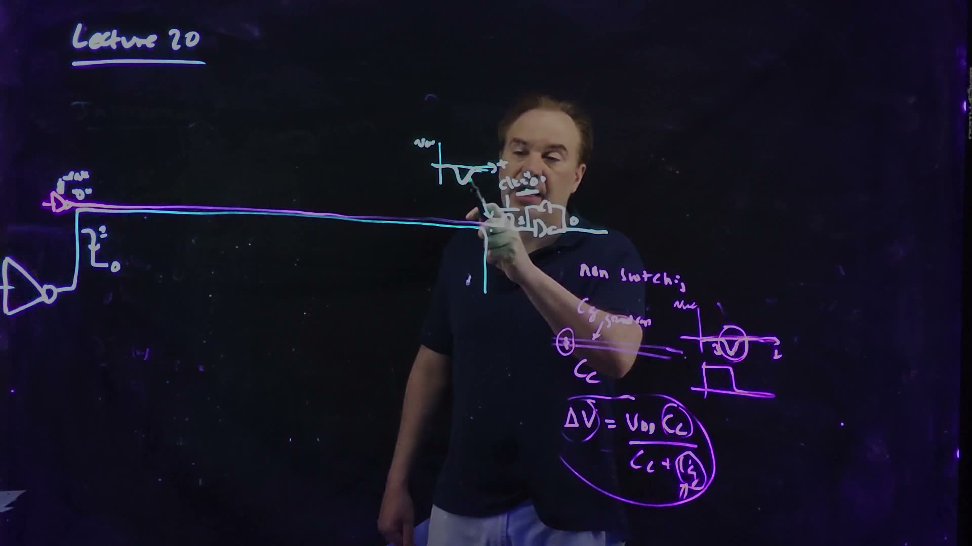
The question. So far a wire’s capacitance has gone “to ground”. But most of it goes to neighbouring wires, and those switch. What does a switching neighbour do to a wire that is supposed to sit still, and how big can the disturbance get?

Ground capacitance and coupling capacitance

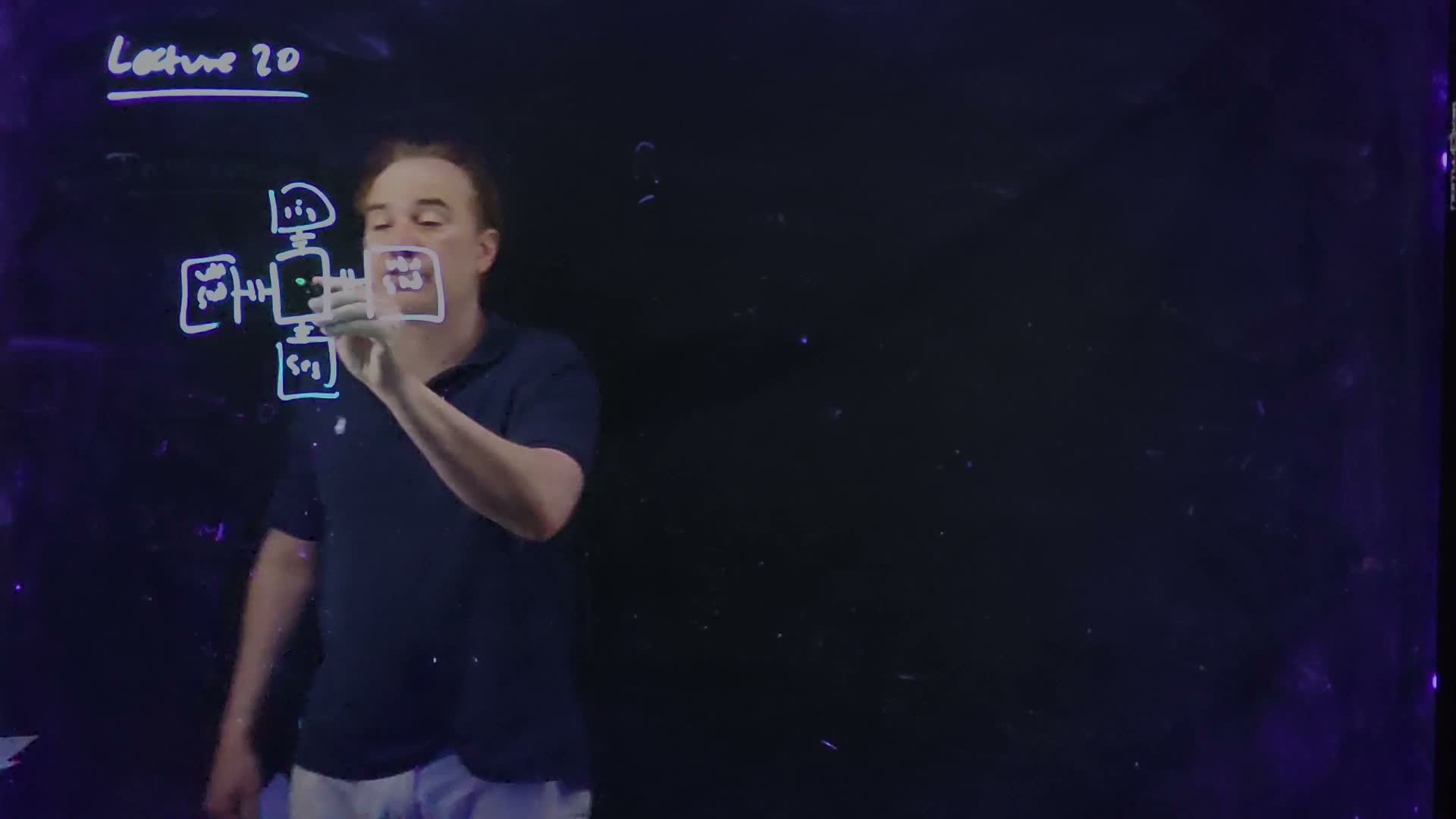
Look at a wire in cross-section (13:00–13:28) board. On the same layer it has neighbours to the left and right; on the layers above and below it may have wires crossing over and under. A wire with neighbours at minimum spacing on all sides is called fully loaded: it has the most capacitance it can have. And nearly all of that capacitance ends on other wires.

A wire and its neighbours in cross-section, redrawn from the board (Lecture20 @ 15:35). The wires run into the page. The side neighbours are power or ground lines, so the capacitance to them is ground capacitance $C_g$ (the board’s “ground caps”). The wires above and below are signals, so the capacitance to them is coupling (floating) capacitance $C_c$ (the board’s “floating/coupling cap”). A signal neighbour that is not switching would also count as ground.

The board (Lecture20 @ 15:35)

Lecture20 @ 15:35The cross-section: ground caps to the power lines at the sides, coupling caps to the signal wires above and below.

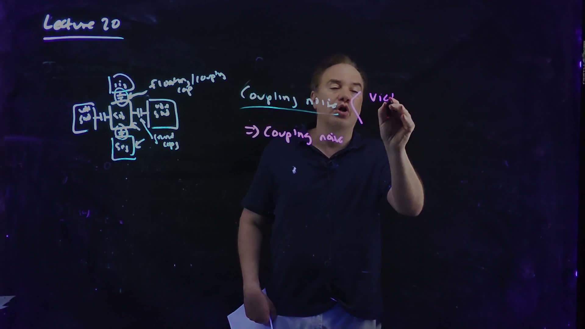
Fair copy of the board above (Lecture20 @ 15:35), mark for mark in its own layout. All black: the lecturer changed pens in mid-topic (the cyan cross-section and heading, the pink line under it), so the colours mark time, not layers. The end of “noise” and of its underline, over the lecturer’s face here, are read from 17:10. “vict” is copied as far as written; by 17:10 it reads “victim”, with “aggressor” under it.

Which neighbours count as what (13:28–14:39, spoken):

• A neighbour that is a $V_{DD}$ or ground line holds still, so the capacitance to it is ground capacitance $C_g$Cg​, whatever the line’s voltage. (For delay, a capacitor to a fixed voltage behaves the same as one to ground.)
• A signal neighbour that is not switching is held by its driver through an on transistor, back to a supply. To first order it holds still too, so it also counts as ground capacitance.
• A signal neighbour that switches is different: the far plate of the capacitor moves. That is coupling (or floating) capacitance $C_c$Cc​.

So $C_g$ and $C_c$ are not properties of the geometry alone. The same capacitor is $C_g$ on a cycle when its neighbour is quiet and $C_c$ on a cycle when it switches.

The coupling glitch

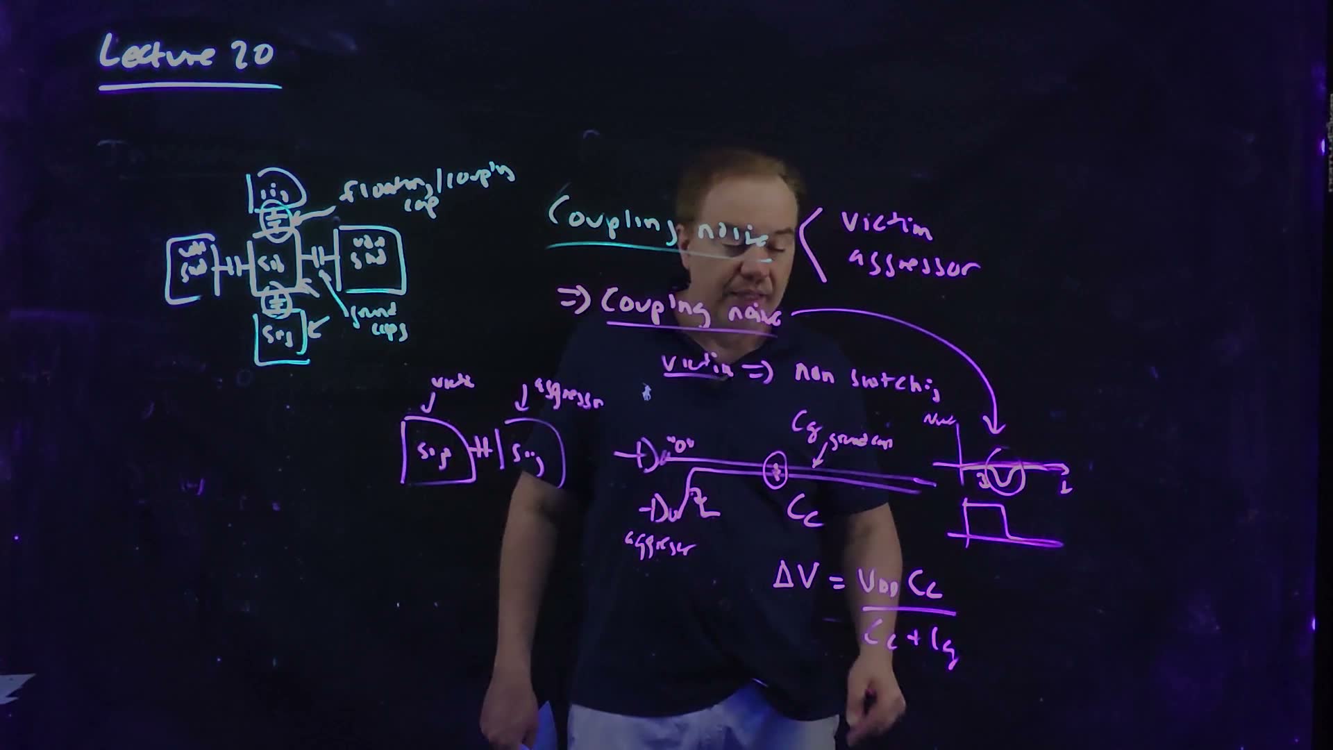
Call the wire we worry about the victim and the switching neighbour the aggressor (15:29). In the coupling-noise case the victim is quiet: its driver holds it, say at 0 (15:55–16:38).

Coupling noise, redrawn from the board (Lecture20 @ 19:55; sign as drawn at 18:25). The victim’s driver holds it at 0. The aggressor beside it falls from $V_{DD}$ to 0 and, through $C_c$Cc​, pulls the victim below 0 for a moment, until the victim’s driver restores it. The worst depth of the glitch is the capacitance divider $\Delta V = V_{DD}\,C_c/(C_c + C_g)$Cg​).

The board (Lecture20 @ 19:55)

Lecture20 @ 19:55The coupling-noise setup, the glitch and its worst size.

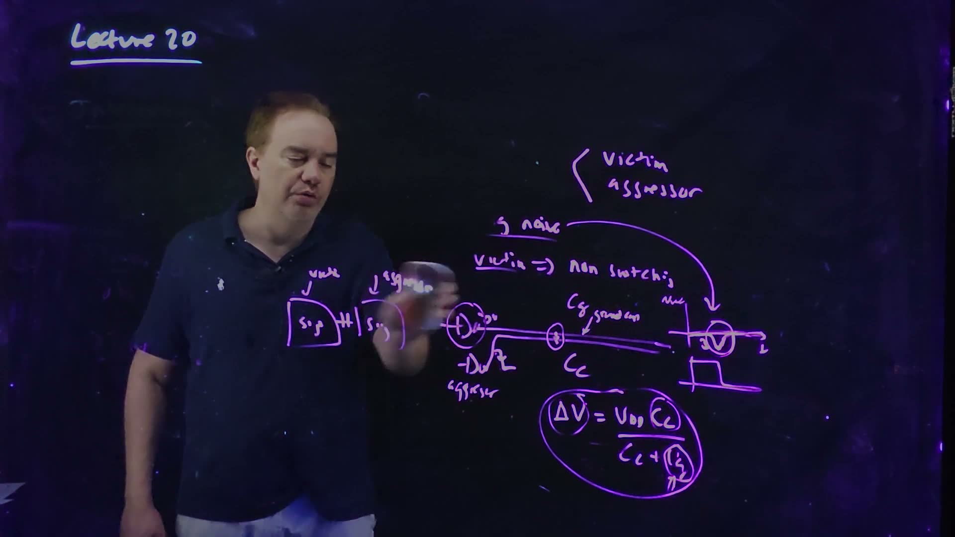
Fair copy of the board above (Lecture20 @ 19:55), mark for mark in its own layout. All black: one pen wrote the whole board. The lecturer is wiping the board from the left: the cross-section and both “Coupling noise” lines are gone, except “g noise” and its underline, and they are left out. The aggressor wire of the two-wire sketch and its “aggressor” label, under his hand and the eraser here, are copied from 19:10.

The worst glitch (board, 17:20–18:32)

1. The aggressor switches. It falls from $V_{DD}$ to 0. Its edge is fast compared with the victim’s driver, so during the edge the driver delivers almost no charge: the victim node is, for that instant, isolated.
2. Charge is shared. The victim node has $C_c$ to the aggressor and $C_g$ to ground. With its charge conserved, a step of $-V_{DD}$ on the far side of $C_c$ moves it by $-V_{DD}\,C_c/(C_c + C_g)$Cg​): the capacitance divider of the Need.
3. The worst depth. So the victim dips below 0 by $\Delta V = V_{DD}\,\dfrac{C_c}{C_c + C_g}$ board. This is the largest glitch: a slower aggressor edge gives the driver time to fight it, and the real peak is smaller.
4. Then it recovers. The victim’s driver, a resistor $R_d$ to ground, pulls the node back to 0 with time constant $R_d(C_c + C_g)$ added.

The glitch as a circuit added. (a) During a fast aggressor edge the victim’s driver $R_d$ (dashed) delivers almost no charge, so the victim node is a capacitance divider between $C_c$ and $C_g$Cg​. (b) Afterwards $R_d$ pulls the node back to 0 with time constant $R_d(C_c + C_g)$Cg​).

The worst coupling glitchboard

$$\Delta V = V_{DD}\,\frac{C_c}{C_c + C_g}$$

Holds when: a quiet victim held by its driver; an aggressor swinging the full V_DD; the aggressor's edge fast enough that the victim's driver delivers no charge during it (so this is an upper bound); C_g is all the victim's capacitance to non-switching conductors

Memorize or derive. Memorize it, and know the two-line derivation: conserve the victim’s charge across the aggressor’s step.

What sets the real peak (18:32–19:20, spoken). Two things. The ratio $C_c/C_g$Cc​/Cg​: if most of the victim’s capacitance is coupling, the glitch approaches $V_{DD}$VDD​; if most is ground, it is small. And the victim’s driver: a strong (“beefy”) driver keeps the peak below the divider value and restores the node fast; a weak one lets the glitch reach nearly the full divider value and keeps it there longer. “These kinds of glitches are worse when the coupling capacitance is large relative to the ground cap or when the driver is weak.” The mirror case is as bad added: a rising aggressor beside a victim held at $V_{DD}$ pushes it above $V_{DD}$ by the same amount.

A worked example

An added example added: $V_{DD} = 1.2$ V, and a victim with $C_c = 40$ fF to an aggressor and $C_g = 120$ fF to everything else.

A 40 fF / 120 fF victim

1. The worst glitch. $\Delta V = 1.2 \times 40/(40 + 120) = 1.2 \times 0.25 =$ 0.30 V below ground.
2. Space the wires. Suppose doubling the spacing halves the coupling to 20 fF and leaves $C_g$ at 120 fF (a stated assumption; the real split depends on the geometry). Then $\Delta V = 1.2 \times 20/140 =$ 0.171 V.
3. Shield instead. Run a grounded line between the two wires: the victim’s capacitance to it is ground capacitance, and the coupling to the aggressor almost disappears. $\Delta V \approx 0$0.
4. The driver’s restore time. For example, a weak driver with $R_d = 5$ kΩ restores the 160 fF node with time constant $5\ \text{k}\Omega \times 160$ fF $=$ 800 ps; a strong one with 500 Ω, in 80 ps.

Traps.

• The wrong numerator. The glitch is the coupling share, $C_c/(C_c + C_g)$Cg​), not $C_c/C_g$ and not $C_g/(C_c + C_g)$Cg​).
• Counting a quiet signal as an aggressor. A neighbour that does not switch this cycle is ground capacitance.
• Expecting a stronger driver to change the divider. It lowers the real peak and shortens the glitch; the charge-sharing bound is the same.

Check yourself What fraction of a victim's capacitance must be coupling to a full-swing aggressor for a worst glitch of V_DD/2?

$C_c/(C_c + C_g) = \tfrac12$21​, so $C_c = C_g$Cg​: half of the victim’s capacitance.

Check yourself A victim has 150 fF in all: 60 fF to an aggressor and 90 fF to quiet neighbours and ground; V_DD = 1.0 V. Find the worst glitch. Then suppose the quiet neighbours also become aggressors, switching the same way at the same moment. What is the bound now?

$\Delta V = 1.0 \times 60/150 = 0.40$ V. If all 150 fF couples to wires that switch together, $C_g = 0$ and the bound becomes the full $V_{DD} = 1.0$ V: only the victim’s driver keeps the glitch smaller.

Check yourself On the board's cross-section, why are the wires above and below the victim coupling capacitance, but the ones beside it ground capacitance?

Because of what they carry, not where they are: the side neighbours are $V_{DD}$/ground lines, which never switch, and the ones above and below are signals that may switch. Swap the labels and the capacitances swap names.

4. When a glitch kills the chip: noise in a latch

You need

The coupling glitch (Section 3). A quiet victim held at 0, next to an aggressor that falls from $V_{DD}$ to 0, dips below ground by up to $\Delta V = V_{DD}\,C_c/(C_c + C_g)$Cg​), worse with a weak victim driver; the driver then restores it.

Coupling noise (Section 3; Lecture20 @ 19:55, redrawn): the falling aggressor pulls the quiet victim below 0. Original figure ↑

When an NFET conducts (Chapter 4). An NFET turns on when its gate is a threshold $V_T$ above its source, and its source is whichever of its two diffusion terminals is lower. Below threshold it still leaks.

The pass-transistor latch (Chapter 13). An NFET pass device, off when its clock is low, feeds a storage node held by a pair of cross-coupled inverters. With the clock low the latch is opaque and must keep its bit, whatever its input does.

The question. A coupling glitch goes away by itself: the driver restores the victim. So why does the lecturer call it “the number two chip killer” (19:45)?

The scenario

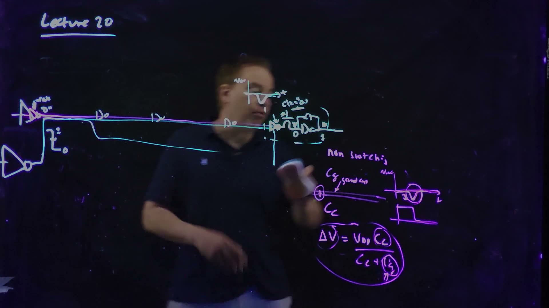
The lecturer draws the case that killed his first microprocessor design (20:16–21:40) board.

The coupling-noise failure, redrawn from the board (Lecture20 @ 22:33 and 23:48). A weak driver holds a very long wire at 0; at its end a pass-transistor latch, its clock low, stores 1 on its storage node (output 0). A big aggressor runs beside the wire for most of its length. When the aggressor falls, the far end of the victim dips below 0; the pass NFET’s wire side becomes its source, $V_{GS} = \Delta V$ reaches $V_T$VT​, and the device drains the storage node: (a) before, (b) after. The latch has flipped although its clock never rose.

The board (Lecture20 @ 23:48)

Lecture20 @ 23:48After the glitch: the latch's stored 1 has become 0 with its clock still at 0.

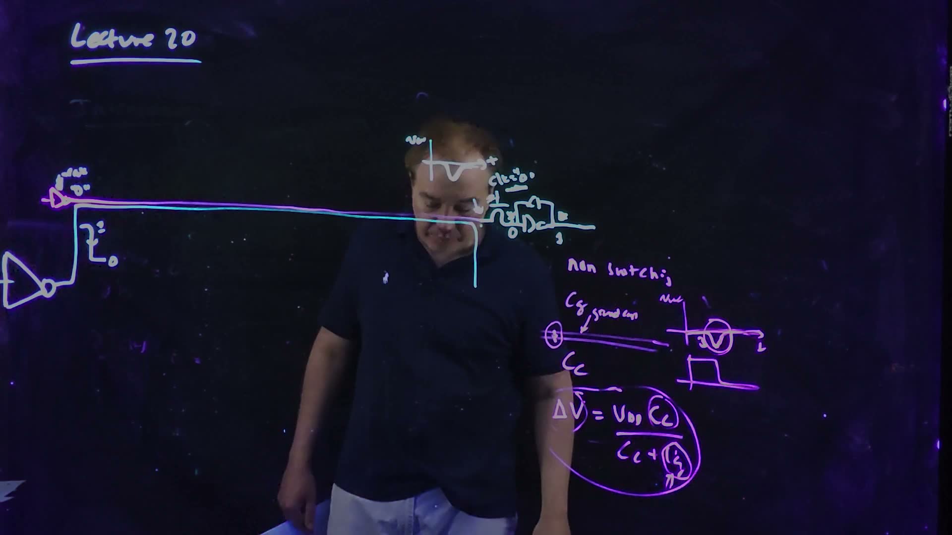
Fair copy of the board above (Lecture20 @ 23:48), mark for mark in its own layout. All black: the pens mark time, not layers. The node values before the glitch (22:33: 1 at the storage node, 0 at the output) are scribbled out above the wire; the values after it, 0 and 1, are written under it. The coupling-noise drawing at the right is what the wiping left of 19:55, so the circle round ΔV and the formula’s ellipse have lost their left edges.

How the latch flips (board and speech, 21:04–23:05)

1. The setup. A very weak driver holds a very long wire at 0. At the far end, a pass-transistor latch is closed (clk = 0) and stores 1 on its storage node, so its output is 0. A big aggressor is coupled to the victim along most of its length.
2. The aggressor falls. The far end of the victim dips below 0. It dips deep: the coupling is large compared with the ground capacitance, the driver is weak, and the long wire’s resistance stands between the far end and its driver (“a decent amount of resistive shielding”, 21:55). Chapter 20’s resistive shielding, which usually only makes a delay estimate a little pessimistic, here works against us.
3. The pass device sees a gate voltage. Its gate is at 0 (clk), its two sides are the storage node at $V_{DD}$ and the wire, now at $-\Delta V$−ΔV. The lower side is the source, so $V_{GS} = 0 - (-\Delta V) = \Delta V$ (22:12–22:47).
4. It conducts. As $\Delta V$ approaches $V_T$ the device leaks heavily; if it reaches $V_T$ it turns on. Either way it drains charge from the storage node toward the wire.
5. The bit flips. If the storage node falls past the inverter’s switching point, the cross-coupled pair regenerates the wrong value: 0 on the node, 1 at the output (23:05). The clock never rose. “This machine is now completely trashed.”

This is a functional failure caused by noise: once a latch holds a wrong value, the chip has failed, and no change of clock frequency brings the bit back. The lecturer ranks it second among chip killers only to the early-mode (short-path) failures of Chapter 14 (19:45).

A compact test for the danger added: the latch is at risk when the worst glitch at its input approaches the pass device’s threshold, $\Delta V \gtrsim V_T$VT​. (Below $V_T$ the device still leaks, so “well below” is the safe side.)

The fixes

The lecture lists four fixes (23:34–24:57):

Four fixes for the latch failure added (spoken at 23:34–24:57; the repeaters drawn on the board at 25:06). (a) Buffer the latch input: an inverter before the pass device. (b) A stronger victim driver. (c) Either space the wires apart or shield them with a ground line between them (one panel shows both). (d) Break the victim wire with repeaters (two are drawn; the board at 25:06 draws three).

1. Never present a bare pass-transistor input. Put an inverter in front of the pass device. The inverter’s input can dip below 0 and nothing happens: its output simply stays high, and the pass device beyond it sees a clean, restored signal. Standard-cell latches always have this input inverter: it removes the mechanism itself.
2. Make the victim’s driver stronger. A beefy driver holds the wire closer to 0.
3. Separate the wires. Route them apart, so they are not coupled over a long length, or put a ground line between them: less $C_c$Cc​, more $C_g$Cg​.
4. Break the wire with repeaters. Each segment is short, so its coupled length is short, and its driver is close to every point of it.

A worked example

Section 3’s example victim added: $V_{DD} = 1.2$ V, $C_c = 40$ fF, $C_g = 120$ fF, and, for example, a pass NFET with $V_T = 0.30$ V.

Is the latch safe?

1. The worst glitch. $\Delta V = 0.30$ V (Section 3).
2. Against the threshold. $V_{GS} = \Delta V = 0.30$ V $= V_T$VT​: with a weak driver, the pass device reaches threshold. The latch is at risk.
3. With the spacing fix. $\Delta V = 0.171$ V, 57% of $V_T$VT​. Below threshold, but the device still leaks during the glitch: safer, not safe by margin.
4. With an input inverter. The dip goes to the inverter’s input, which is already at 0 and only goes further below its switching point. Its output stays at $V_{DD}$VDD​, and the latch never sees the glitch. Nothing flips, whatever $\Delta V$ is.

Traps.

• The NFET’s “usual” source. Its source is whichever diffusion is lower, here the wire, not a fixed terminal.
• “It recovers, so it is harmless.” A storage node does not recover: once the pair regenerates, the wrong bit stays.
• Slowing the clock. The failure happens while the clock is off.

Check yourself Why does an inverter at the latch input stop the failure, even though the glitch is just as large?

The glitch now lands on an inverter’s gate. Its input dips from 0 to below 0, further from its switching point, so its output stays high. The pass device beyond sees that restored output, not the glitch, and its $V_{GS}$ never rises.

Check yourself With Section 3's numbers (V_DD = 1.2 V, C_g = 120 fF) and V_T = 0.30 V, how small must C_c be for the worst glitch to stay at half of V_T?

Set $1.2\,C_c/(C_c + 120) = 0.15$0.15: $1.2\,C_c = 0.15\,C_c + 18$18, so $C_c = 18/1.05 = 17.1$ fF, less than half the original 40 fF.

Check yourself Which of the four fixes also makes the victim faster when it switches?

The stronger driver and the repeaters (Section 2) both speed up the victim’s own transitions. Spacing helps too, a little, by lowering its capacitance. The input inverter adds a gate delay at the latch.

5. Noise on delay: simultaneous switching and the Miller factor

You need

Coupling and ground capacitance (Section 3). A victim wire has $C_g$ to everything that holds still and $C_c$ to an aggressor that switches.

The wire’s neighbours (Section 3; Lecture20 @ 15:35, redrawn): ground capacitance to the power lines, coupling capacitance to the signals. Original figure ↑

A capacitor’s current added (circuits). $I = C\,dV/dt$CdV/dt, where $V$ is the voltage across the capacitor: the difference between its two plates.

Delay and load (Chapter 20). A driver of resistance $R_d$ charging a load $C$ has Elmore delay $R_dC$Rd​C, the course’s estimate of the 50% delay: the delay is proportional to the capacitance the driver must charge.

The question. Now let the victim switch too, at the same moment as the aggressor (“simultaneous switching”, 26:06). How much does the coupling capacitance load the victim’s driver: as much as a ground capacitor, more, or less?

Zero, one or two times C_c

The lecturer’s way to think about it (26:24–28:10, spoken): count the voltage change across $C_c$ while the victim rises from 0 to $V_{DD}$VDD​. That change, times $C_c$Cc​, is the charge the victim’s driver must push through it.

The Miller factor added (spoken at 26:24–28:10). The victim rises by $V_{DD}$VDD​. (a) Aggressor quiet: the voltage across $C_c$ changes by $V_{DD}$VDD​, so $C_c$ loads the victim like a ground capacitor. (b) Same direction: both plates rise together, the voltage across $C_c$ does not change, and it draws no charge: it is as if it were not there. (c) Opposite direction: the voltage across $C_c$ changes by $2V_{DD}$2VDD​, twice the charge: it loads like $2C_c$2Cc​.

Three aggressor cases

1. The aggressor is quiet. One plate rises by $V_{DD}$VDD​, the other holds: the voltage across $C_c$ changes by $V_{DD}$VDD​, and the victim’s driver supplies $C_cV_{DD}$Cc​VDD​. “If the aggressor is quiet, it’s gonna look like C.”
2. It switches the same way, at the same time. Both plates rise together, so the voltage across $C_c$ stays at 0 and no current flows through it (26:55–27:10). “It almost looks like that capacitor isn’t there at all.”
3. It switches the opposite way. One plate rises by $V_{DD}$ while the other falls by $V_{DD}$VDD​: the voltage across $C_c$ changes by $2V_{DD}$2VDD​, so the driver supplies $2C_cV_{DD}$2Cc​VDD​. “It’s going to look like 2C” (27:16–28:10): a Miller amplification, like a feedback capacitor across an inverting amplifier.

The victim's effective loadadded

$$C_{eff} = C_g + m\,C_c, \qquad m \in \{0,\ 1,\ 2\}$$

Holds when: victim and aggressor swing the full V_DD at the same time (the same edge rate); m = 0 same direction, 1 aggressor quiet, 2 opposite direction (the three cases are the lecture's, spoken); a first-order picture: real edges overlap only partly, so m lies between these values

Memorize or derive. Memorize the three cases (0, $C_c$Cc​, $2C_c$2Cc​); derive them in one line each from the voltage change across $C_c$Cc​.

The waveform: a later 50% point, and a step

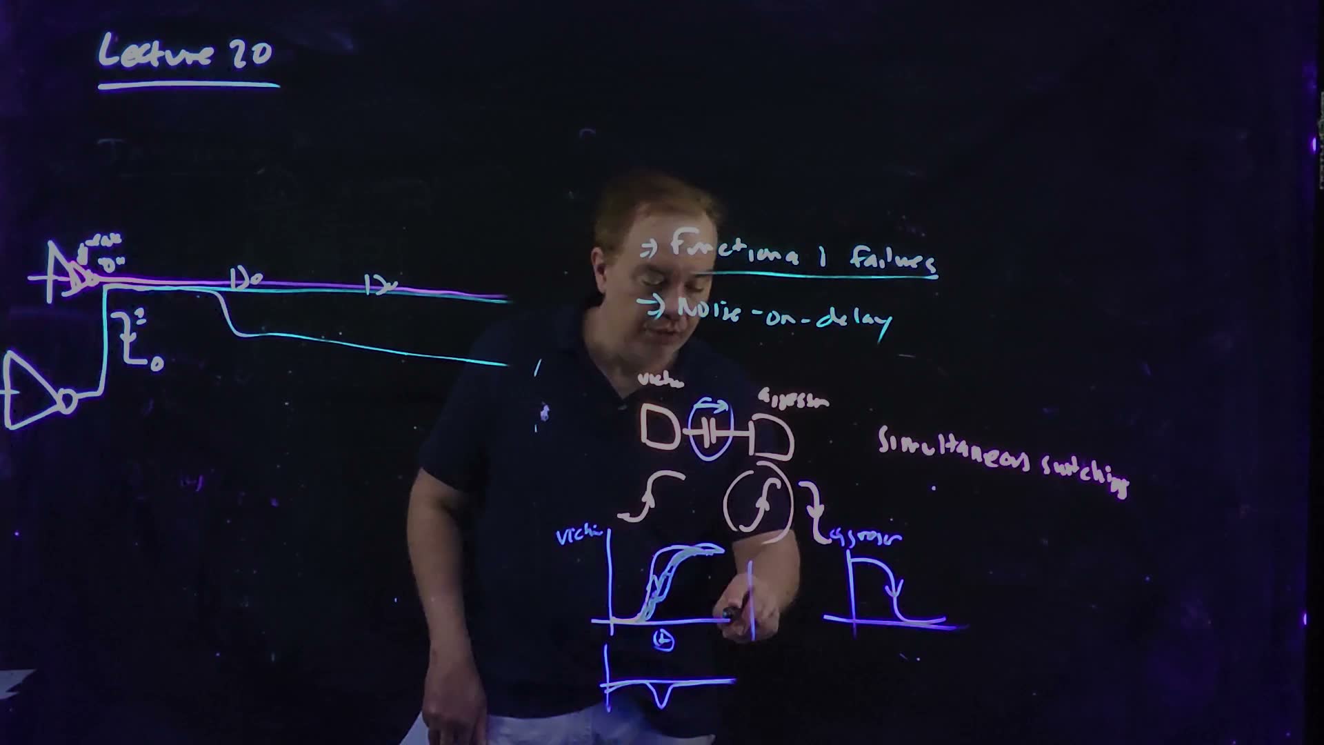
The three cases oversimplify. The lecture’s second picture is a superposition (28:33–30:55) board. It is not exact, because the victim’s driver is not a linear circuit, “but it’s useful to analyze it that way nonetheless”.

Noise on delay, redrawn from the board (Lecture20 @ 30:30 and 31:57). (a) The victim’s own rising waveform. (b) The aggressor falling at the same time. (c) Their superposition: the glitch the aggressor would put on a quiet victim (inset) is added to the victim’s rise. The sum crosses 50% later, by $\Delta t$Δt, and may show a step partway up. The waveforms are a sketch.

The board (Lecture20 @ 31:57)

Lecture20 @ 31:57The superposition: victim, aggressor, glitch, and the delayed, stepped victim waveform.

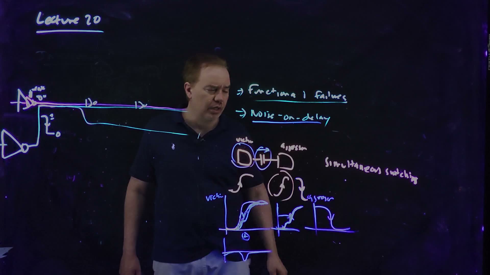
Fair copy of the board above (Lecture20 @ 31:57), mark for mark in its own layout. All black: the pens mark time, not layers. The left half is what the wiping left of the latch board (23:48–25:06): the driver, both aggressor wires and two of the three repeaters; the third repeater and the latch were wiped.

1. Add two pieces. Take the victim’s waveform as its driver would produce it alone, and add the dip the falling aggressor would put on a quiet victim (Section 3). The dip pulls the rise down while it is rising, so the sum reaches the 50% point later (30:07–30:36): the new delay.
2. A step. Depending on the timing, the sum can even have a small step, a shoulder, partway up. Waveforms like this are “very common” on coupled nets, not the clean saturated ramps of Chapter 6 (30:36–31:29).

Timing tools handle it by putting margins on the coupling capacitance (30:55–31:29). The worst case for a long-path (setup) check is the opposite-switching aggressor, $m = 2$2. The same-direction case, $m = 0$0, makes the victim faster, and that is the worst case for a short-path (hold) check, the early mode of Chapter 14 added.

A worked example

An added example added: a victim driver of, for example, $R_d = 1$ kΩ, with $C_g = 100$ fF and $C_c = 50$ fF to one aggressor. Take the delay as the Elmore estimate $R_dC_{eff}$Rd​Ceff​.

The victim's delay window

1. Aggressor quiet ($m = 1$m=1). $C_{eff} = 150$ fF, delay $1\ \text{k}\Omega \times 150\ \text{fF} =$ 150 ps.
2. Same direction ($m = 0$m=0). $C_{eff} = 100$ fF: 100 ps.
3. Opposite ($m = 2$m=2). $C_{eff} = 200$ fF: 200 ps.
4. The window. The same wire’s delay lies anywhere from 100 to 200 ps, depending on what its neighbour does: ±33% around the quiet value. A timing tool must use 200 ps for setup and 100 ps for hold.

Traps.

• $2C_c$ for a quiet aggressor. Doubling is the opposite-direction case; a quiet aggressor counts once.
• Ignoring the speed-up. The same-direction case is not harmless: it is the hold-time worst case.
• Taking superposition as exact. It is a picture of why the 50% point moves; the driver is nonlinear.

Check yourself Which aggressor case is the worst for a setup (long-path) check, and which for a hold (short-path) check?

Setup: the opposite direction, $m = 2$2, the slowest victim. Hold: the same direction, $m = 0$0, the fastest.

Check yourself In the example, give the victim a second aggressor of 50 fF on its other side (C_g stays 100 fF). What is the range of R_dC_eff between both aggressors switching with it and both against it?

Both with it: $C_{eff} = 100$ fF, 100 ps. Both against it: $100 + 2 \times 50 + 2 \times 50 = 300$ fF, 300 ps. The window has widened to a factor of 3.

Check yourself Why can the superposed waveform have a step partway up?

The glitch is a short dip. If it arrives while the victim is rising, it pulls the rise down for a moment and then lets go, so the sum rises, nearly stalls while the dip is at its deepest, and rises again.

6. Wire inductance and the current’s return path

You need

Inductance added (circuits). A current $I$ around a loop makes a magnetic flux $\Phi$ through the loop; if the current changes, the changing flux induces a voltage around the same loop, $V = d\Phi/dt$dΦ/dt. For a given loop the flux is proportional to the current, $\Phi = LI$LI, which defines its inductance $L$L: so $V = L\,dI/dt$LdI/dt. A larger loop area holds more flux for the same current, so it has more inductance.

Where a gate’s current goes (Chapter 6). To charge its output wire, an inverter’s PFET draws charge from $V_{DD}$ and pushes it onto the wire’s capacitance; that capacitance ends on other conductors (Section 3), and the charge has to get back to the supply that sent it. Discharging runs the loop the other way, through the NFET to ground.

Decoupling capacitance, for this section only: a capacitor between $V_{DD}$ and ground near the driver, through which a current loop can close (Sections 10–12 teach it).

Where the supply’s current flows (Section 10): from the package through its inductances, with a decap between the chip’s rails. Original figure ↑

The question. Resistance and capacitance belong to a wire. Inductance does not: it belongs to a loop of current. So what is “the inductance of a wire” on a chip, and how can a designer know it?

A current loop

The lecture builds the loop on a driver and a long wire (33:28–36:00) board.

The current loop of a driven wire, redrawn from the board (Lecture20 @ 39:54). Switching the wire high, the driver pulls current from the supply and sends it down the signal wire into the wire’s capacitance; the current returns along a ground line and closes through the on-chip decoupling capacitance (left) back to the supply. The hatched area between signal and return holds the loop’s magnetic flux, which sets its inductance: $V = d\Phi/dt = L\,dI/dt$LdI/dt. The return takes the path of least $\lvert R + j\omega L\rvert$jωL∣.

The board (Lecture20 @ 39:54)

Lecture20 @ 39:54The loop: signal out, ground return back, closed through the decap; the flux area and V = L dI/dt.

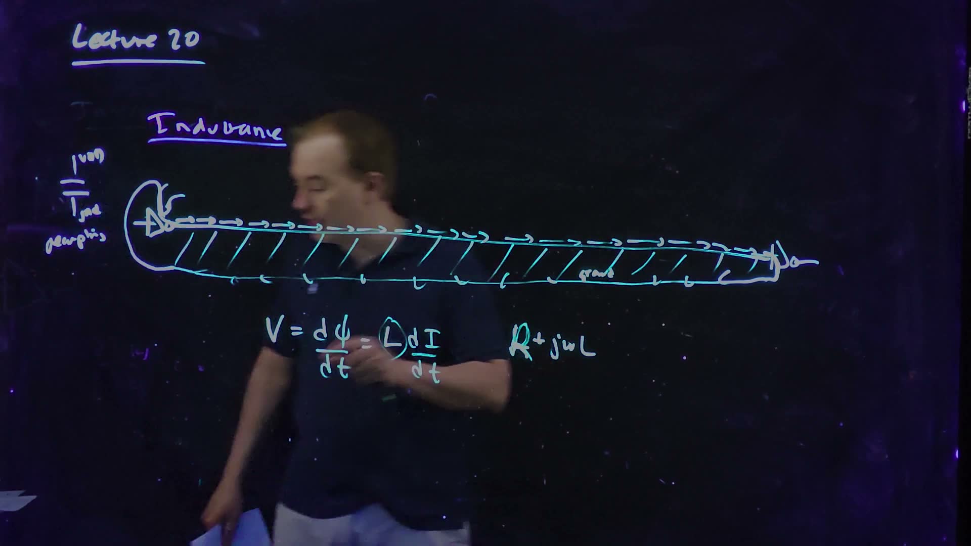
Fair copy of the board above (Lecture20 @ 39:54), mark for mark in its own layout. All black: the pale pen (the decap and its labels), the violet heading and the cyan loop and equations mark the order of writing, not separate layers. The board writes the flux as $\psi$ψ. The lecturer stands in front of the middle of the wire here; its arrows and hatching there, and the second “=” under his hand, are copied from 39:07. The wire is copied as drawn, closing in on the return line towards the receiver; the equations are levelled.

1. Out along the signal. Switching the net high, the driver pulls current out of the supply and pushes it down the wire, charging the wire’s capacitance (33:48–34:23).
2. Back along a return. “The current doesn’t just disappear”: it comes back, for example along a ground wire beside the signal, and closes through the on-chip decoupling capacitance to the supply (34:23–35:56). It is one loop.
3. Flux and inductance. The loop encloses an area. The current’s magnetic field links it, and a changing current induces $V = d\Phi/dt = L\,dI/dt$ around it (36:00–36:28) board.
4. The return decides. “If this loop is bigger … the inductance is bigger. If this return is closer … the inductance is smaller” (36:28–36:53). The inductance of the wire depends entirely on where its current returns.

The return path depends on frequency

“It gets even hairier” (37:04). The current has many possible return paths, and it takes the one that minimizes its impedance, $R + j\omega L$ board (37:26):

Where the return current flows added (spoken at 37:04–39:49). (a) At DC the return takes the least resistance, perhaps out through the package; as the frequency rises it moves onto the chip, and at the highest frequencies it takes the closest line, which gives the least inductance. (b) A controlled return: a ground and a power line placed right beside the signal, as a ground plane does on a circuit board.

• At DC, $\omega L$ is nothing and the current takes the least resistance. That may be out through a bond wire or a C4 bump to the package and back, a path with an enormous loop and so enormous inductance (37:40).
• As the frequency rises, $\omega L$ dominates, and that path stops being taken: the return moves onto the chip.
• At the highest frequencies it takes the return that makes the loop smallest: the line closest to the signal (38:12). These are the frequencies that matter for fast edges, so this is the return that sets a fast signal’s inductance.

Controlling the return

Not knowing where the return is makes the inductance unpredictable (38:40). Circuit boards put a ground plane under the signals, so the return always flows right under the trace. Chips have no ground plane, but can do the same locally (39:15–39:49): put a power or a ground line directly next to the signal. It becomes the return path, and the signal’s inductance is controlled and predictable. Wires whose inductance matters are routed this way, and a power grid (Section 9) gives every signal such lines nearby.

Where the return current flows (this section’s figure). Original figure ↑

Which return, when added. On the return-paths figure: a slowly varying current (a supply droop that builds over microseconds, say) returns through the least resistance, possibly through the package. A fast clock edge, whose frequency content reaches tens of gigahertz, returns through the ground line beside it, and its inductance is that of the small loop.

Traps.

• “The wire’s inductance per unit length” quoted without saying where the return is. Inductance belongs to the loop.
• One return for all frequencies. The DC current and the edge current of the same wire can return in different places.

Check yourself Why does a grid of V_DD and ground lines (Section 9) also lower the inductance of the signal wires routed through it?

Every signal then has a power or ground line close beside it, which a fast current takes as its return. The loop it forms is small, so the signal’s inductance is small, and known.

Check yourself A signal's loop has, for example, 0.5 nH with its return right beside it and 2 nH with its return three tracks away. Its edge changes the current by 10 mA in 20 ps. Find L dI/dt for both returns. Why is the far one larger?

$dI/dt = 10\ \text{mA}/20\ \text{ps} = 5 \times 10^8$ A/s. Near return: $0.5\ \text{nH} \times 5 \times 10^8$ A/s $= 0.25$ V. Far return: $2\ \text{nH} \times 5 \times 10^8$ A/s $= 1.0$ V. The far return encloses a larger loop area, so the same current makes more flux: more inductance, more induced voltage.

7. When inductance matters: RC, LC and the slew time

You need

When resistance matters (Chapter 20). A wire’s resistance can be ignored, and the wire treated as a plain capacitor, when its Elmore delay is small compared with the slew time of the signals on it; it matters when the Elmore delay is comparable to the slew or longer. A long uniform wire’s intrinsic Elmore delay is $\tfrac12\mathcal{R}\mathcal{C}\ell^2$ (Chapter 20’s $\tfrac12\mathcal{R}\mathcal{C}L^2$21​RCL2; $\ell$ is its $L$L).

A loop’s inductance (Section 6). With a controlled return beside it, a wire has a known inductance per unit length $\mathcal{L}$L.

The current loop (Section 6; Lecture20 @ 39:54, redrawn). Original figure ↑

A transmission line added (background). A wire whose resistance is small enough behaves as a lossless line, $\mathcal{L}$ and $\mathcal{C}$ per unit length: a signal travels along it at the speed $1/\sqrt{\mathcal{L}\mathcal{C}}$1/LC​, so its delay is the time of flight, $\sqrt{\mathcal{L}\mathcal{C}}\,\ell$LC​ℓ. On chip that speed is the speed of light in the dielectric.

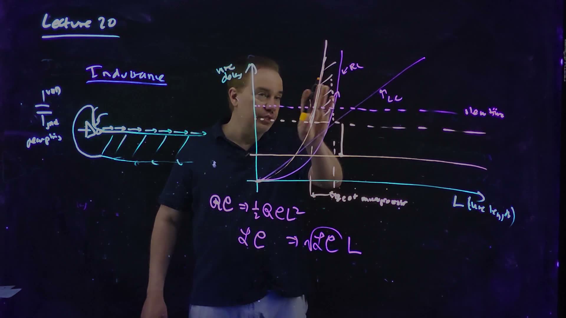
The question. Which wires need their inductance in the analysis? The lecture answers with one picture: three times plotted against the wire’s length (39:51–49:22).

Three curves against length

The picture (board, 40:14–42:21)

1. The RC delay. A uniform wire’s Elmore delay, $\tfrac12\mathcal{R}\mathcal{C}\ell^2$ board, plotted against the length is a parabola.
2. The LC delay. If the wire behaves as a transmission line, its delay is the time of flight, $\sqrt{\mathcal{L}\mathcal{C}}\,\ell$ board: a straight line. At short lengths the line lies above the parabola (a parabola starts flat), and beyond a crossover the parabola wins.
3. The slew time. A horizontal line. A wire whose delay is below the signals’ slew time does not need R or L at all: it is a capacitor.

Which delay is the “real” one? The larger of the two governs added: a signal cannot arrive before its time of flight, however small the RC; and when the RC delay is the longer, the wire is so resistive that the slow diffusion of charge, not the travelling wave, sets the delay. So at a given length the wire is capacitive if both are below the slew time; a transmission line if the LC delay is above both the RC delay and the slew time; an RC line if the RC delay is the largest.

How the window opened

How the inductance window opened, redrawn from the board (Lecture20 @ 42:57 and 44:32). (a) The half-micron world: the RC curve reaches the slew time only at the chip’s own size, so every on-chip wire is capacitive. (b) Scaling: slew times fell (arrow down) and scaled wires got more resistive (the RC curve moves left); then copper and wider, thicker top-level wires pushed the RC curve back to the right.

The board (Lecture20 @ 42:57)

Lecture20 @ 42:57The half-micron world: the RC curve meets the slew time only at the size of the microprocessor. The board writes L for the wire's length; this chapter writes ℓ.

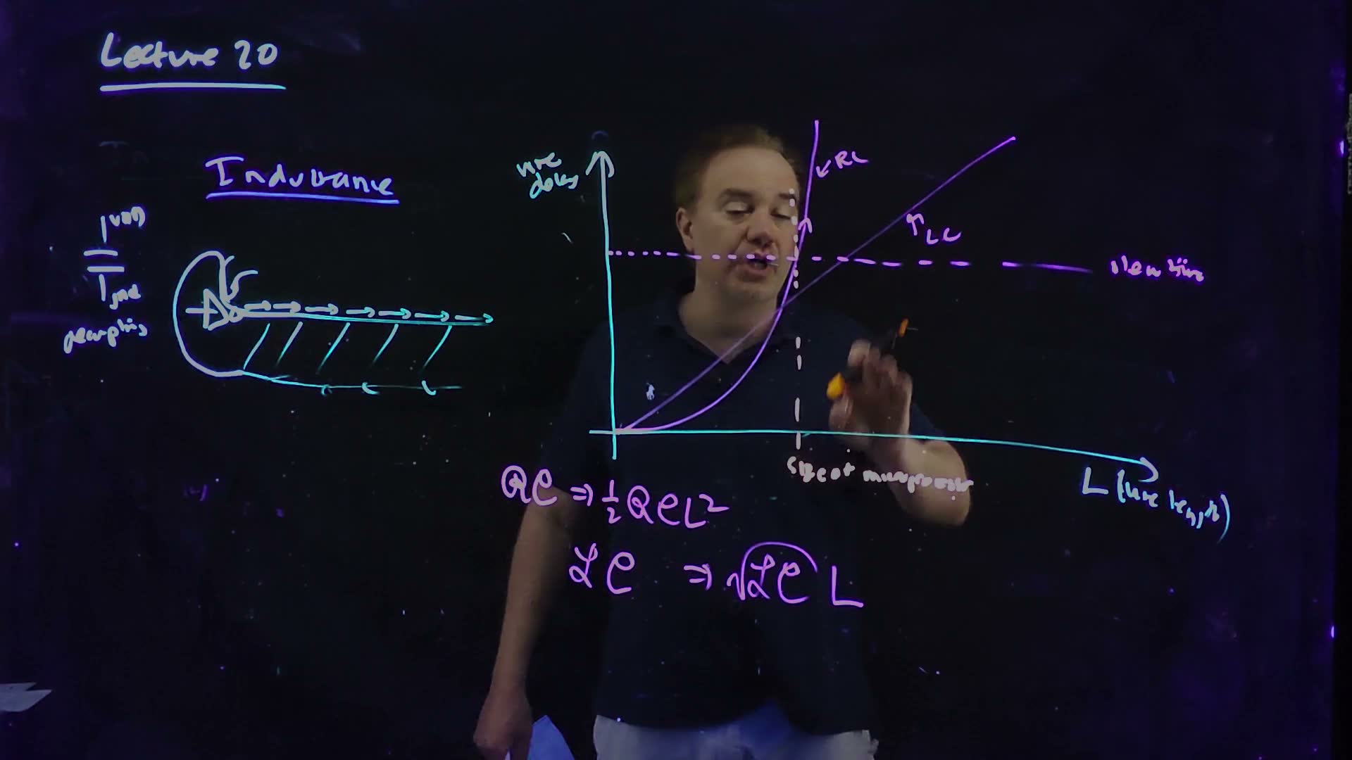
Fair copy of the board above (Lecture20 @ 42:57), mark for mark in its own layout. All black: the cyan loop and axes, the violet curves and formulas and the pale pink chip-size marker follow the order of writing, not separate layers. The board writes $L$ for the wire’s length. “Size of microprocessor”, under the lecturer’s hand here, is copied from 43:42; the parabola and the dotted slew line behind his head, from 41:42 and 43:42. The plot is levelled; the board’s axis droops to the right.

The lecture tells the history on this picture (42:21–46:34), as the figure shows. In the half-micron world every on-chip wire was a capacitor; from about a quarter micron to 90 or 65 nm many wires needed RC analysis, as they still do. Copper and wide, thick top-level wires then pushed RC back while slew times kept falling, and together they opened a window of lengths where the LC curve lies above both the RC curve and the slew line.

When inductance matters, redrawn from the board (Lecture20 @ 49:37). Short wires, whose delays are below the slew time, are capacitive (C). Between the length $\ell_1$ where the time of flight reaches the slew time and the crossover $\ell^{*}$ where the RC delay overtakes it, the wire is a transmission line and its inductance matters (LC). Longer wires are RC lines again.

The board (Lecture20 @ 49:37)

Lecture20 @ 49:37Today's picture: capacitance only, then a transmission-line window, then RC.

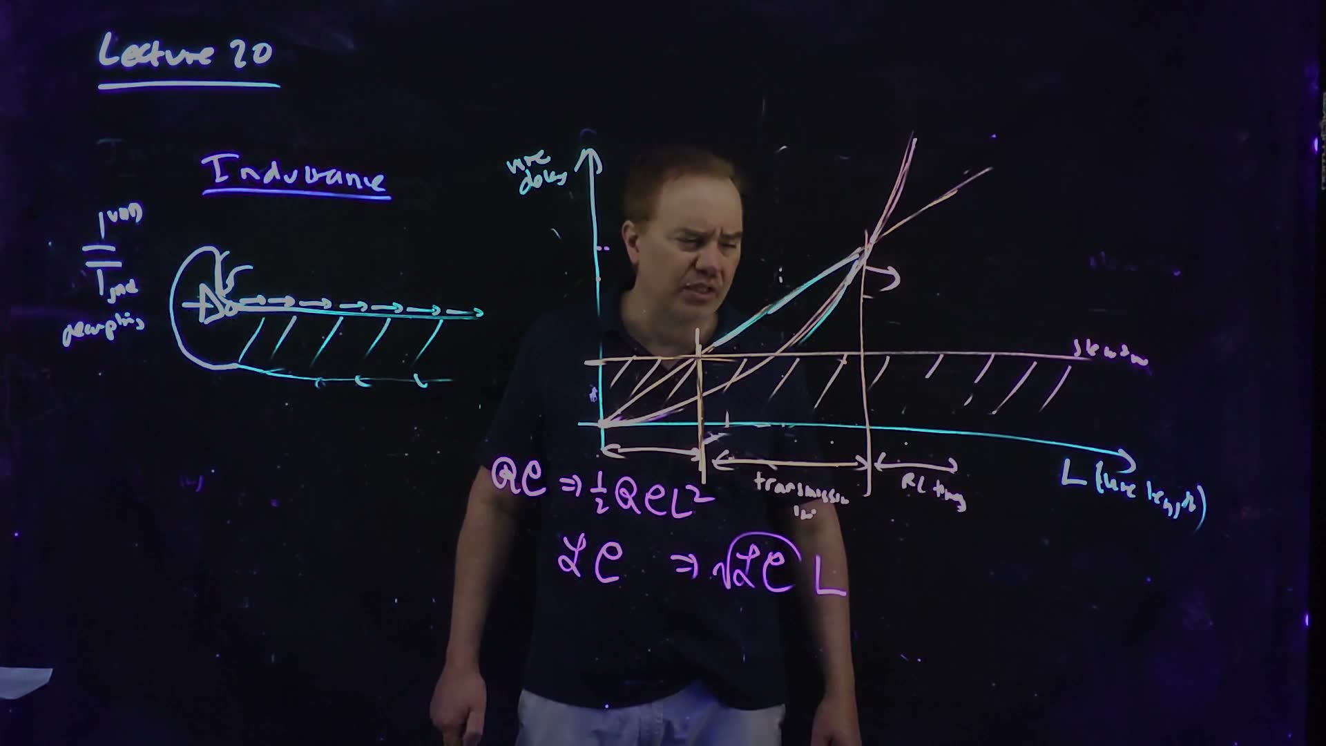
Fair copy of the board above (Lecture20 @ 49:37), mark for mark in its own layout. Magenta is the pale pink pen (it looks peach here): the picture redrawn at 45:08 to “show where we are today”, with its curves, slew line, hatching, verticals, ranges and labels. Black is the rest: the cyan loop and axes and the violet formulas kept from 42:57. The last label reads “RC thing”. The hatching and the curves near the vertical axis, behind the lecturer’s head, are copied from 47:37 and 48:52. Each curve is drawn twice on the board and copied once.

A good thing, not a bad one (46:35–49:22). On a microprocessor’s clock tree the lecturer’s team widened wires until the RC estimate came out less than the time of flight, which is impossible: inductance was setting the delay. Forbidding such wires would be “completely nonsense”: they are “the fastest you can go on that wire, which is basically time of flight”. Clock nets and long lines are now analysed with their inductance.

Where the window is

The board leaves the crossover unnamed. Two lines of algebra place it added:

The crossover and the test

1. Equate the two delays. $\tfrac12\mathcal{R}\mathcal{C}\ell^2 = \sqrt{\mathcal{L}\mathcal{C}}\,\ell$ gives the crossover $\ell^{*} = \dfrac{2\sqrt{\mathcal{L}\mathcal{C}}}{\mathcal{R}\mathcal{C}}$RC2LC​​. Below $\ell^{*}$ the time of flight is the larger delay; above it, the RC delay.
2. The delay there. Put $\ell^{*}$ into the LC delay: $\sqrt{\mathcal{L}\mathcal{C}} \cdot 2\sqrt{\mathcal{L}\mathcal{C}}/(\mathcal{R}\mathcal{C}) = 2\mathcal{L}/\mathcal{R}$2L/R. At the crossover both delays equal $2\mathcal{L}/\mathcal{R}$2L/R, and that is the largest delay a wire can have while it is still a transmission line.
3. The test. The window exists only if the time of flight can exceed the slew time before $\ell^{*}$ℓ∗, that is, if $t_{slew} < 2\mathcal{L}/\mathcal{R}$2L/R. If the slew time is much longer than $2\mathcal{L}/\mathcal{R}$2L/R, inductance does not matter at any length.
4. The same test in frequency. A wire’s $j\omega\mathcal{L}$ equals its $\mathcal{R}$ at $\omega = \mathcal{R}/\mathcal{L}$R/L, the inverse of the time constant $\mathcal{L}/\mathcal{R}$L/R. Inductance matters only if that frequency lies within the signal’s frequency content, roughly up to $1/t_{slew}$1/tslew​. A signal that is too slow to reach $\omega = \mathcal{R}/\mathcal{L}$ sees only resistance.
5. No slew time given? Two ways out. (a) Compare the wire’s length with $\ell^{*}$ℓ∗: a wire much longer than $\ell^{*}$ is an RC line whatever the slew, because the larger delay governs. (b) Estimate the slew from the gates: an edge on the chip takes at least about one FO1 delay, $\tau_{inv}$τinv​, so if $\tau_{inv} \gg 2\mathcal{L}/\mathcal{R}$ inductance does not matter.

RC and LC wire delaysboard

$$t_{RC} = \tfrac12\,\mathcal{R}\mathcal{C}\,\ell^2 \qquad\qquad t_{LC} = \sqrt{\mathcal{L}\mathcal{C}}\;\ell$$

Holds when: a uniform wire, per-unit-length ℛ, 𝒞 and ℒ (with a controlled return), length ℓ; RC is the intrinsic Elmore delay, LC the lossless time of flight

The inductance windowadded

$$\ell^{*} = \frac{2\sqrt{\mathcal{L}\mathcal{C}}}{\mathcal{R}\mathcal{C}}, \qquad t_{RC}(\ell^{*}) = t_{LC}(\ell^{*}) = \frac{2\mathcal{L}}{\mathcal{R}}$$

Inductance can matter only if

$$t_{slew} \lesssim \frac{2\mathcal{L}}{\mathcal{R}}$$

Holds when: a uniform wire with per-unit-length ℛ, 𝒞 and ℒ and a controlled return; RC is the intrinsic Elmore delay and LC the lossless time of flight; an order-of-magnitude comparison (the curves are estimates, and the slew time is not sharp)

Memorize or derive. Memorize the two delays (the board’s). Derive the window: equate them, solve for $\ell^{*}$ℓ∗, substitute back, compare with the slew time.

A worked example

An added example added: a wide top-level wire with, for example, $\mathcal{R} = 5$ Ω/mm, $\mathcal{C} = 0.2$ pF/mm and $\mathcal{L} = 0.25$ nH/mm (with a return beside it). Since 1 Ω × 1 pF = 1 ps, the RC delay is $\tfrac12 \times 5 \times 0.2\ \ell^2 = 0.5\,\ell^2$ ps with $\ell$ in mm.

Does this wire need its inductance?

1. The time of flight. $\sqrt{\mathcal{L}\mathcal{C}} = \sqrt{0.25 \times 10^{-9} \times 0.2 \times 10^{-12}}$ s/mm $= 7.07$ ps/mm, so $t_{LC} = 7.07\,\ell$ ps.
2. The crossover. $\ell^{*} = 2 \times 7.07/(5 \times 0.2) = 14.1$ mm. Check: $2\mathcal{L}/\mathcal{R} = 2 \times 0.25\ \text{nH}/5\ \Omega = 0.1$ ns $= 100$ ps, and indeed $t_{RC}(14.1) = 0.5 \times 14.1^2 = 100$ ps and $t_{LC}(14.1) = 100$ ps.
3. With a 50 ps slew. 50 ps is below 100 ps, so a window exists. The time of flight passes 50 ps at $50/7.07 = 7.07$ mm. Wires from 7.07 to 14.1 mm of this kind need their inductance; shorter ones are capacitors, longer ones RC lines.
4. With a 200 ps slew. The time of flight would reach 200 ps only at 28.3 mm, beyond $\ell^{*}$ℓ∗, where the RC delay has already taken over. 200 ps is above $2\mathcal{L}/\mathcal{R} = 100$ ps: no window. Inductance never matters for this wire at these slews.

The worked example, computed from $t_{RC} = \tfrac12\mathcal{R}\mathcal{C}\ell^2$ and $t_{LC} = \sqrt{\mathcal{L}\mathcal{C}}\,\ell$ added with $\mathcal{R} = 5$ Ω/mm, $\mathcal{C} = 0.2$ pF/mm, $\mathcal{L} = 0.25$ nH/mm. With a 50 ps slew the shaded window, 7.07 to 14.14 mm, needs inductance. With a 200 ps slew (dashed) there is none: the crossover’s delay, $2\mathcal{L}/\mathcal{R} = 100$ ps, is below it.

Traps.

• Comparing RC with LC and forgetting the slew. Both can be negligible: then the wire is just a capacitor.
• Calling low resistance a problem. The window appears because the wire is fast; the time of flight is the speed limit.
• Mixed units. With $\mathcal{R}$ in Ω/mm and $\mathcal{C}$ in pF/mm, $\ell$ must be in mm; 1 Ω × 1 pF = 1 ps, and $\sqrt{\text{nH} \cdot \text{pF}}$ per mm is 31.6 ps/mm.

Check yourself Which two changes over the technology generations opened the inductance window?

Falling slew times (faster gates) and lower wire resistance on the top layers (copper, wide and thick wires), which pushed the RC curve to the right and left the time of flight as the longer delay over a range of lengths.

Check yourself For the example wire, what slew time makes the window just disappear, and what is ℛ/ℒ in rad/s?

The window closes when $t_{slew} = 2\mathcal{L}/\mathcal{R} = 100$ ps. And $\mathcal{R}/\mathcal{L} = 5\ \Omega/0.25\ \text{nH} = 2 \times 10^{10}$ rad/s: signals must have frequency content of that order (edges of a few tens of picoseconds) for the inductance to show.

Check yourself Why can no wire's real delay be less than its time of flight, however small its RC delay?

The time of flight is how long the signal takes to travel the wire’s length at the speed of light in the dielectric. Nothing reaches the far end sooner; an RC estimate below it only shows that the RC model no longer describes the wire.

8. Supply noise: IR drop, L dI/dt, and what it does to delay

You need

Ohm’s law and inductance. A current $I$ through a resistance $R$ drops $IR$IR; a changing current through an inductance $L$ induces $L\,dI/dt$ (Section 6).

A gate’s delay depends on its supply (Chapter 5). A gate’s delay is about charge over current, $\tau \propto CV_{DD}/I$CVDD​/I. With a fully velocity-saturated device at full overdrive, $I \propto V_{DD} - V_T$VT​, so $\tau \propto V_{DD}/(V_{DD} - V_T)$VT​): a lower supply gives less current and a slower gate. The fs1 practice page works this model on FN10-6.

A wire’s RC delay does not depend on the supply (Chapter 20): $\mathcal{R}$ and $\mathcal{C}$ are set by the metal and the dielectric.

The supply’s path onto the chip (Section 10; Lecture20 @ 57:57, redrawn): the package’s inductances, the circuits’ current and the decap. Original figure ↑

The question. Every gate assumes $V_{DD}$ above ground, steady. What makes the real supply move, and what does a gate do when it does?

Two kinds of supply noise

The goal (50:52–51:44): power at $V_{DD}$VDD​, ground at 0, and above all the difference between them “rock solid”. It is not: the difference moves, and that is power-supply noise board. It has two parts (51:44–52:35):

• DC: IR drop. The chip draws an average current, and the power network has resistance, so the supply at the circuits sits lower than at the pins: the supply has “collapsed or drooped”. Its cause is the network’s resistance.
• AC: $L\,dI/dt$ noise. The chip’s demand for current changes quickly, clock edge by clock edge, and the network and the package have inductance: the transient current induces a voltage that makes the supply fluctuate. Its cause is inductance.

A power and ground grid added, after the board (Lecture20 @ 55:29). $V_{DD}$ and ground straps alternate on every metal layer, each layer in its preferred direction, joined by vias. From the supply pads at the edge there are many parallel paths to any point $X$ (thick arrows), so the resistance and the inductance to every point are low. A signal routed between a $V_{DD}$ and a ground strap has its current return beside it.

The board (Lecture20 @ 55:29)

Lecture20 @ 55:29Supply noise, DC (IR drop) and AC (L dI/dt), and the grid that fights both.

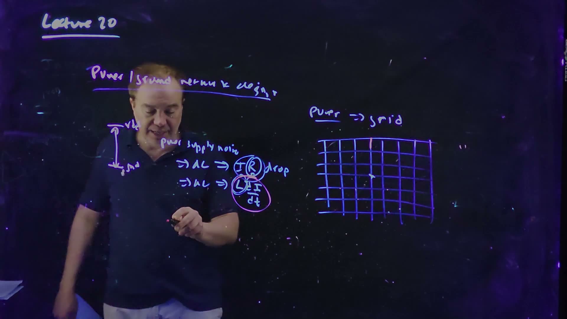
Fair copy of the board above (Lecture20 @ 55:29), mark for mark in its own layout. Magenta is the violet-pink pen: the large circle round dI/dt, the start of the L dI/dt layer that continues at 57:57 with the off-chip circuit. Everything else is black: the pale title and arrow, the blue noise lines with their rings, and the grid. † The board writes the first line’s “dc” as “ac”; the lecture says DC noise is the IR drop (51:44–52:25), so it reads “⇒ dc ⇒ IR drop”. “Power/ground”, “vdd” and “gnd”, behind the lecturer’s head here, are read from 57:57. The title is levelled; the grid is copied as drawn.

Either kind hurts the circuits in two ways (52:35–53:02): they “depend on this potential to define their delay”, and on it “to determine logic one and logic zero values”. A moving supply disturbs delays, and a large one can cause functional failures. Hence the two remedies of the next sections: a network with low resistance and low inductance (Section 9), and charge stored close to the circuits (Section 10).

What a droop does to delay

The lecture states the effect on delay in words. A first-order rule turns it into a number added:

From a supply change to a delay change

1. The sensitivity. Define how strongly a delay $\tau$ depends on the supply, as a ratio of fractional changes: $S = \dfrac{V_{DD}}{\tau}\,\dfrac{\partial\tau}{\partial V_{DD}}$τVDD​​∂VDD​∂τ​. It is negative: a lower supply makes a gate slower. With the velocity-saturated model of the Need, $S = 1 - V_{DD}/(V_{DD} - V_T) = -V_T/(V_{DD} - V_T)$VT​).
2. A small change. Replace the derivative by a difference: $\Delta\tau/\tau \approx S\,\Delta V_{DD}/V_{DD}$SΔVDD​/VDD​, so $\Delta\tau \approx S\,\tau\,\dfrac{\Delta V_{DD}}{V_{DD}}$SτVDD​ΔVDD​​. A droop ($\Delta V_{DD} < 0$ΔVDD​<0) with $S < 0$ gives $\Delta\tau > 0$0: slower.
3. Only the silicon. In a path made of gates and wires, only the gates’ delay $\tau_{silicon}$ depends on the supply; the wires’ RC part does not. Apply the rule to the gate delays only.
4. Jitter. If the supply moves from one clock edge to the next, the delay of every buffer on the clock’s path moves with it, so the clock edge itself arrives earlier or later from cycle to cycle. That cycle-to-cycle wander of an edge is jitter (taught with clock distribution in Chapter 23, Lecture 22). A droop that is the same on every cycle only slows the path; one that comes and goes makes it jitter.

Supply-induced delay changeadded

$$\Delta\tau \approx S\,\tau_{silicon}\,\frac{\Delta V_{DD}}{V_{DD}}, \qquad S = \frac{V_{DD}}{\tau}\,\frac{\partial\tau}{\partial V_{DD}}$$

Holds when: a small supply change (a few percent, up to about 10%); S defined as (V_DD/τ)(∂τ/∂V_DD) at the nominal supply; apply it to the gates' (silicon) delay only, not to wire RC

Memorize or derive. Derive: it is the first term of a Taylor expansion of $\tau(V_{DD})$τ(VDD​), written with fractional changes because that is how $S$ is defined.

A worked example

Added numbers added, all for example: $V_{DD} = 1.2$ V.

Droops and their cost

1. IR drop. The chip draws 2 A on average through a power network whose effective resistance to the circuits is 25 mΩ: $IR = 2 \times 0.025 =$ 50 mV, 4.2% of 1.2 V.
2. L dI/dt. The demand jumps by 1 A in 100 ps. Through one 1 nH bond wire that would induce $1\ \text{nH} \times 1\ \text{A}/100\ \text{ps} =$ 10 V: impossible, the supply would collapse. Through 100 such wires in parallel (10 pH): 0.1 V. That is why Section 10’s remedies exist.
3. The sensitivity. With a velocity-saturated device and $V_T = 0.4$ V: $S = -0.4/(1.2 - 0.4) = -0.5$−0.5.
4. The delay change. A clock path has 1 ns of buffer delay and 300 ps of wire delay, and the supply droops by 5%. The buffers slow by $\Delta\tau = (-0.5)(1000\ \text{ps})(-0.05) =$ 25 ps; the wires do not change. The path goes from 1300 to 1325 ps.
5. As jitter. If the droop comes and goes from cycle to cycle, the clock edge at the end of the path wanders over about 25 ps.

Check. The exact model gives a little more: $V_{DD}/(V_{DD} - V_T)$ is $1.2/0.8 = 1.5$ at 1.2 V and $1.14/0.74 = 1.541$ at 1.14 V, a 2.7% increase, so the buffers slow by 27 ps rather than 25. The first-order rule is slightly low because the delay curves upward as the supply falls.

Traps.

• The whole path. The sensitivity applies to the gates, not to the wires’ RC.
• The sign. A droop with a negative $S$ lengthens the delay.
• “10% supply noise”. Say whether it means a droop of 10%, a rise, or ±10%; a supply swinging ±10% moves an edge over twice the range of a one-sided 10% droop.

Check yourself Which kind of supply noise does a larger on-chip decap reduce, and which does a lower-resistance grid reduce?

Decap supplies transient charge locally, so it reduces the AC, $L\,dI/dt$LdI/dt, part. A lower-resistance grid reduces the DC, IR-drop, part (and, with more parallel paths, the on-chip inductance too).

Check yourself A path has 600 ps of buffer delay with S = −1.2, and 400 ps of wire. The supply droops by 3%. What is the path's new delay?

Only the buffers change: $\Delta\tau = (-1.2)(600)(-0.03) = 21.6$ ps. The path goes from 1000 ps to 1021.6 ps.

Check yourself Why does a supply that sags by the same amount on every cycle slow a clock path but cause no jitter?

Jitter is the edge’s change from cycle to cycle. A constant sag makes every buffer slower by the same amount on every cycle, so every edge is late by the same time: a longer latency, but no wander.

9. Power and ground grids

You need

The two kinds of supply noise (Section 8). IR drop comes from the network’s resistance; $L\,dI/dt$ noise from its inductance. Both must be small at every point where circuits draw current.

Parallel paths added (circuits). $N$ equal resistances in parallel give $R/N$R/N; $N$ equal inductances in parallel, if their mutual coupling is ignored, about $L/N$L/N.

A controlled return (Section 6). A power or ground line right beside a signal carries the signal’s return current, which keeps the signal’s loop, and its inductance, small.

Return paths (Section 6): the nearest line carries a fast signal’s return. Original figure ↑

Layout image (Chapter 9). Each metal layer has a preferred routing direction, alternating up the stack.

The question. How should the power and ground wiring itself be built, so that the supply at every circuit stays close to $V_{DD}$VDD​?

Grids on every layer

The lecture’s answer is a grid (53:02–54:02) board. Power and ground are both grids, strapped on every metal layer, metal 1, metal 2, metal 3, metal 4 and up, each layer “following layout image” (its preferred direction), all the way to the top level. The figure in Section 8 shows one.

A power and ground grid (Section 8): many parallel paths to every point. Original figure ↑

Why a grid (board and speech, 53:37–55:00)

1. Thick top layers carry the current across the chip. The top levels of interconnect are thick and wide, so they give “very low resistance paths” to distribute the power and cut the IR drop.
2. Many paths to every point. Feed the grid from its periphery: to reach the centre there are many paths, so “lots of resistors, lots of inductors in parallel”. Every point of the grid has low resistance and low inductance to the supply.
3. The capacitance helps. A grid adds capacitance between its $V_{DD}$ and ground lines. On a signal that would be a cost; on the supply it is decoupling capacitance (Section 11): a benefit.
4. The one cost. It uses a lot of metal: routing tracks that signals cannot use. “There’s nothing we can do about that.”
5. Returns for signals. Every signal has a $V_{DD}$ or ground line nearby: the controlled return of Section 6.

So “grids are the only way to do power and ground distribution” (54:31): their only weakness is routing, and nobody distributes power and ground any other way.

Memorize the reasons, in order of importance: (1) low resistance and low inductance, from many parallel (redundant) paths to every point; (2) the grid’s own metal–metal capacitance is decap; (3) controlled current returns for the signals. The cost: routing resources.

A worked example

An added example added, with illustrative numbers: one strap from the edge pads to the chip’s centre has 2 Ω; the circuits at the centre draw 1 A.

One strap against a grid

1. One strap. $IR = 1\ \text{A} \times 2\ \Omega = 2$ V: more than the whole supply. One path cannot do it.
2. Forty paths. A grid giving 40 such paths in parallel has $2/40 =$ 50 mΩ, so the drop is 50 mV.
3. The inductance too. If each path also has some inductance $L$L, forty in parallel give about $L/40$L/40: the same grid lowers the $L\,dI/dt$ noise on chip.

Traps.

• Capacitance as a cost. On the supply network it is decap; the only cost is routing.
• Only the resistance. The key reason is low resistance and low inductance.

Check yourself Give three reasons why grids are preferred for power and ground distribution, the most important first.

(1) Many parallel paths to every point give low resistance and low inductance, so low IR drop and low $L\,dI/dt$ noise. (2) The grid’s $V_{DD}$-to-ground metal capacitance is built-in decoupling capacitance. (3) Its lines give every signal a nearby current return, lowering the signals’ inductance. The cost is routing tracks.

Check yourself With the example's 2 Ω paths, how many in parallel keep the IR drop at the centre below 1% of a 1.0 V supply at 1 A?

1% of 1.0 V is 10 mV, so the resistance must be at most 10 mΩ: $2\ \Omega/N \le 0.01\ \Omega$0.01 Ω, $N \ge 200$ paths.

10. Off-chip inductance and decoupling capacitance

You need

$L\,dI/dt$ noise (Sections 6 and 8). A changing current through an inductance induces $V = L\,dI/dt$LdI/dt; on the supply path it makes the supply at the circuits droop while the current changes.

Parallel inductances (Section 9). $N$ equal paths in parallel have about $1/N$ of one path’s inductance.

Charge sharing (Section 3). Two capacitors joined with no other current conserve their total charge; the result is a capacitance divider, as in the coupling glitch.

The capacitance divider of the coupling glitch (Section 3); the decap calculation below is the same divider. Original figure ↑

The question. The supply comes onto the chip through the package. What does the package’s inductance do when the chip’s current changes fast, and how much on-chip capacitance does it take to stop it?

The package’s inductance

The supply’s path onto the chip, redrawn from the board (Lecture20 @ 57:57). The off-chip supply reaches the circuits through the package’s inductances $L$ (bond wires), one in each rail. A fast change $dI/dt$ in the circuits’ current induces $L\,dI/dt$ across them, so the chip’s own supply droops to $V_{DD} - \Delta V$ added. The decoupling capacitance $C_{decap}$ between the chip’s rails supplies the transient charge locally.

The board (Lecture20 @ 57:57)

Lecture20 @ 57:57The bond-wire inductances, the transient current and the decoupling capacitance.

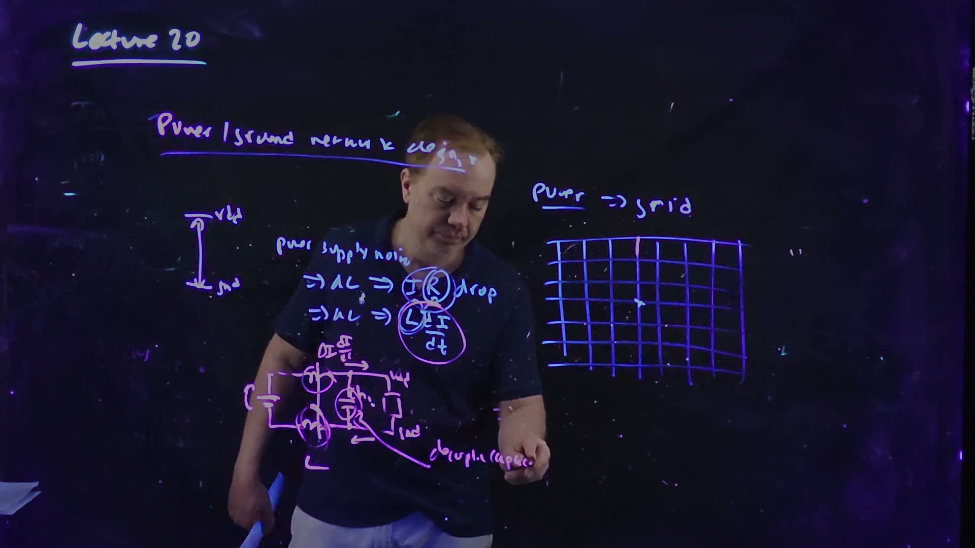
Fair copy of the board above (Lecture20 @ 57:57), mark for mark in its own layout: the 55:29 board, with the off-chip circuit added below. Magenta is the violet-pink pen, the L dI/dt layer: the large circle round dI/dt, the circuit with its circled bond-wire inductances, the current arrows and the label. Everything else is black. † The first line’s “ac” should read “dc”, as at 55:29. The title’s last word, “design”, behind the lecturer’s head here, is read from 55:29. The label is copied as far as written; by 59:16 it reads “decoupling capacitance”.

Three remedies for off-chip inductance (board and speech, 55:12–58:26)

1. The problem. A wire-bonded chip connects to its supply through bond wires, which “can have very substantial inductances”. When the chip pulls a large transient current, a large $dI/dt$ through them gives a voltage droop on chip.
2. Many connections. A wire-bonded chip never has one $V_{DD}$ and one ground bond wire: it has many of each, in parallel, which divides the inductance (56:27–56:55).
3. Lower-inductance connections. C4 (flip-chip) bumps, “little solder bumps” that join the chip face-down to the package, have much less inductance than a bond wire (57:25; packaging is in Chapter 22).
4. Decoupling capacitance. Put capacitance between $V_{DD}$ and ground on the chip: decap for short (57:25–58:26). It is “a charge reservoir to meet the transient current demands of the chip without requiring that that current be pulled through the off-chip connections”. The decap delivers the fast part of the current; the current through the package inductance then changes slowly, its $dI/dt$ is small, and so is the droop. “Have as much on-chip decoupling capacitance as you possibly can.”

How much decap: charge sharing

How large must the reservoir be? A charge balance answers it added.

Sizing a decap by charge sharing added. (a) Before a clock edge the decap holds $C_{decap}V_{DD}$ and the load that is about to switch, $C_{sw}$Csw​, is empty. (b) The edge connects them (the drivers’ PFETs turn on) faster than the package’s inductance can deliver charge (dashed), so they share the decap’s charge: the supply drops by $\Delta V = V_{DD}\,C_{sw}/(C_{sw} + C_{decap})$Cdecap​), the same divider as a coupling glitch.

The droop of one switching event

1. Before. The decap is charged to $V_{DD}$VDD​: charge $C_{decap}V_{DD}$Cdecap​VDD​. The load that is about to switch high (the clock net, say) is at 0: $C_{sw}$ holds nothing.
2. During the edge. The load’s drivers connect it to the supply. The edge is faster than the package can respond, so all the charge comes from the decap.
3. After. Both capacitors sit at the same voltage $V_{DD} - \Delta V$ΔV, and the charge is conserved: $C_{decap}V_{DD} = (C_{decap} + C_{sw})(V_{DD} - \Delta V)$ΔV).
4. The droop. Solve: $\dfrac{\Delta V}{V_{DD}} = \dfrac{C_{sw}}{C_{sw} + C_{decap}}$Csw​+Cdecap​Csw​​. It is the coupling glitch’s divider again, with $C_{sw}$ in the place of $C_c$Cc​.
5. The target. For a droop of at most a fraction $\varepsilon$ of the supply: $C_{sw}/(C_{sw} + C_{decap}) \le \varepsilon$ε, so $C_{decap} \ge C_{sw}\,(1 - \varepsilon)/\varepsilon$ε)/ε. For 10%, nine times the switching load.

Decap for an allowed droopadded

$$\frac{\Delta V}{V_{DD}} = \frac{C_{sw}}{C_{sw} + C_{decap}} \qquad\Longrightarrow\qquad C_{decap} \ge C_{sw}\,\frac{1 - \varepsilon}{\varepsilon}$$

Holds when: ε is the allowed droop as a fraction of V_DD; the switching load starts discharged and charges within one edge, faster than the package can resupply, so its charge comes from the decap alone; the decap is close enough that its series resistance does not shield it (Section 11); one switching event (the package refills the decap between edges)

Memorize or derive. Derive: conserve the decap’s charge across the edge (two lines), then solve for $C_{decap}$Cdecap​.

A worked example

An added example added: a load of 2 nF switches on every clock edge, and the supply may droop by at most 5%.

Sizing the decap

1. The target. $C_{decap} \ge 2\ \text{nF} \times (1 - 0.05)/0.05 = 2 \times 19 =$ 38 nF.
2. Check. $2/(2 + 38) = 0.05$0.05: a 5% droop, as required.
3. What it costs. At, for example, 10 fF/µm² of thin-oxide MOS capacitance (Section 12), 38 nF is $38 \times 10^6\ \text{fF}/(10\ \text{fF}/\mu\text{m}^2) = 3.8 \times 10^6$ µm² $=$ 3.8 mm² of decap: real chip area, which is why the implicit decap of Section 11 is welcome.

Traps.

• $C_{decap} = C_{sw}/f$Csw​/f. That forgets that the load keeps part of the shared charge; the divider has $C_{sw} + C_{decap}$ below.
• Forgetting the conditions. The estimate is per edge and assumes the package refills the decap between edges; a decap far away, behind series resistance, cannot deliver the charge in time.

Check yourself Why do C4 bumps reduce the droop even with the same decap?

Their inductance is much lower, so the package can deliver more of the transient current itself, sooner, with less $L\,dI/dt$ across the connections. The decap then has to carry less of the edge.

Check yourself The example's chip has 38 nF of decap, and its switching load grows to 3 nF. What is the droop now, and how much more decap restores 5%?

$3/(3 + 38) = 7.3\%$7.3%. For 5%: $C_{decap} \ge 3 \times 19 = 57$ nF, so 19 nF more.

11. Where decap comes from: implicit and explicit, and series resistance

You need

Decap’s job (Section 10). A capacitance between $V_{DD}$ and ground on chip that supplies the fast part of the circuits’ current, so that the current through the package changes slowly.

Junction capacitance (Chapter 3). A reverse-biased pn junction is a capacitor: its depletion region is the dielectric.

Wells (Chapter 5). The n-well, which holds the PFETs, is tied to $V_{DD}$VDD​; the $p$-substrate is tied to ground; the junction between them is reverse biased.

An RC time constant (Chapter 20). A capacitor $C$ behind a resistance $R_s$ cannot respond faster than about $R_sC$Rs​C.

The decap’s place (Section 10; Lecture20 @ 57:57, redrawn). Original figure ↑

The question. Where does a chip’s decap come from? Some of it is there whether or not anyone adds it, and the rest is added on purpose. And is all decap equally useful?

Implicit decap: three sources

The lecturer first says “extrinsic and intrinsic”, then corrects himself: explicit and implicit decap are the better terms (59:14–59:35) board. Implicit decap “is just there”: it comes with the design. Explicit decap is added on purpose (Section 12).

The three sources of implicit decap, redrawn from the board (Lecture20 @ 64:23). (a) Metal–metal: neighbouring $V_{DD}$ and ground lines of the grid. (b) n-well: each well, at $V_{DD}$VDD​, against the substrate, at ground. (c) Non-switching circuits: a quiet inverter holding a 1 connects the next gate’s input capacitance through its on PFET to $V_{DD}$VDD​. (d) Each is a capacitor behind a series resistance $R_s$Rs​: lowest for metal–metal, higher for the well (well and substrate resistance) and for quiet circuits (the on transistor).

The board (Lecture20 @ 64:23)

Lecture20 @ 64:23The decap board: explicit and implicit, the three implicit sources, and the series resistance of each.

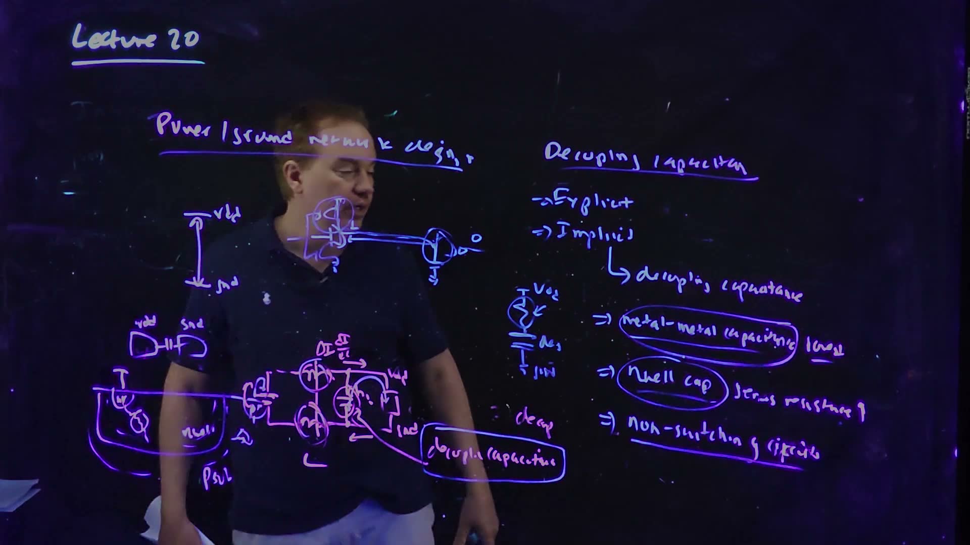
Fair copy of the board above (Lecture20 @ 64:23), mark for mark in its own layout. Magenta is the pink pen: the off-chip circuit drawn at 57:57 (the supply, the two circled inductors and “L”, the circled decap, the circuits, “ΔI dI/dt”, vdd, gnd and the current arrows) with its label “decoupling capacitance”, and “decap”. Black is the violet and blue pens: the title, the vdd–gnd arrow, the wire pair, the n-well, the quiet inverter pair, the R–C model and the list, and over the pink circuit the arc from the decap to the circuits and the box round its label. These two pens mark the order of writing, not a separate layer. The supply-noise lines and the grid of 55:29–57:57 were wiped by 61:44. The lecturer’s head covers the middle of the heading and the inverter pair in this frame; both are copied from 65:08 and checked against 63:48. The headings and the list are levelled; the board’s lines drift down to the right.

1. Metal–metal capacitance (60:29–61:00). In the power grid itself, $V_{DD}$ and ground lines run side by side; the capacitance between them is decap. (This is the second reason for grids in Section 9.)
2. n-well capacitance (61:05–61:35). Every n-well sits at $V_{DD}$ and the substrate around it at ground, so the well-to-substrate junction is a capacitor between the supplies. All the n-wells on the chip together are a large decap.
3. Non-switching circuits (61:35–62:34). Take an inverter driving another, both quiet: the first outputs 1, so its PFET is on, and the second’s gate capacitance hangs from $V_{DD}$ (through that PFET) to ground. Every gate that is not switching this cycle lends its input capacitance as decap.

Series resistance shields a decap

Each of these has a resistance in series with it (62:34–64:18) board, and that changes how useful it is:

• The bigger the series resistance, the more it shields the capacitor: a fast current transient sees the resistance first, and the capacitor can only respond on time scales longer than its $R_sC$Rs​C. So a decap behind a large resistance is “less effective, particularly for fast transients”.
• Metal–metal has the lowest series resistance: it is wired directly into the grid.
• The n-well’s charge must come through the well’s and the substrate’s resistance, from the tap to the junction under the whole well: more.
• Quiet circuits reach the supply through an on transistor: more.

All three still contribute “significant decoupling capacitance”.

The SOI lesson (64:50–65:35). The lecturer once worked on a design mapped straight from bulk CMOS to silicon-on-insulator (Chapter 24). SOI has no n-wells, so all the n-well decap vanished, and “suddenly we had a lot more noise on the power supply than we had before”. That is how much decap the wells quietly provide in an ordinary bulk process.

Memorize the four sources (implicit: metal–metal, n-well, non-switching circuits; explicit: thin-oxide MOS decap, Section 12) and which has the lowest series resistance (metal–metal).

A worked example

Illustrative numbers added.

Which decap can catch a 100 ps edge?

1. n-well decap. 1 nF behind an effective 0.5 Ω: $R_sC = 0.5\ \Omega \times 1\ \text{nF} =$ 0.5 ns. A current edge of 100 ps is over long before this decap responds: it helps with slower fluctuations, little with the edge.
2. Metal–metal decap. 1 nF behind 0.05 Ω: $R_sC =$ 50 ps, fast enough for a 100 ps edge.
3. The point. Count the decap that can respond in the time of the edge, not just the capacitance.

Traps.

• The grid’s resistance as a “source”. The sources are capacitances: metal–metal, n-well, quiet circuits, explicit MOS decap.
• Switching gates as decap. Only the gates that are quiet in that cycle hold their input capacitance across the supply.

Check yourself Two decaps, for example: A is 2 nF behind 0.1 Ω, B is 0.5 nF behind 0.02 Ω. A load of 50 pF switches in a 50 ps edge. Which decap can serve the edge, and what droop does it give on its own?

Time constants: A, $0.1\ \Omega \times 2\ \text{nF} = 200$ ps, too slow for a 50 ps edge; B, $0.02\ \Omega \times 0.5\ \text{nF} = 10$ ps, fast enough. With B alone, Section 10’s divider gives $0.05/(0.05 + 0.5) = 9.1\%$ droop: the bigger decap is the less useful one at this speed, and B is too small on its own.

Check yourself Name four sources of on-chip decoupling capacitance, and say which has the lowest series resistance.

Implicit: metal–metal capacitance between the grid’s $V_{DD}$ and ground lines, n-well-to-substrate junctions, and the input capacitance of non-switching circuits (held through their drivers’ on transistors). Explicit: thin-oxide MOS capacitors. The metal–metal capacitance has the lowest series resistance.

Check yourself Why did the bulk design ported to SOI have more supply noise, and which decap would you count on there instead?

SOI has no n-wells, so the n-well junction decap, a large share of a bulk chip’s implicit decap, disappeared. What is left is the metal–metal capacitance and the quiet circuits, so the design needs more explicit MOS decap to make up the loss.

12. Building explicit decap: MOS unit cells, pinholes and fuses

You need

The MOS capacitor (Chapter 5). With the channel inverted, a MOSFET’s gate capacitance is its full $C_{ox}WL$Cox​WL, the most capacitance per area a chip can build, because the gate oxide is the thinnest dielectric on it.

Series resistance (Section 11). A decap behind a resistance $R_s$ responds only on time scales longer than about $R_sC$Rs​C.

A distributed RC line (Chapter 20). A conductor with resistance and capacitance spread along it has a time constant that grows as the square of its length: $\tfrac12\mathcal{R}\mathcal{C}\ell^2$21​RCℓ2.

Implicit decap and its series resistance (Section 11; Lecture20 @ 64:23, redrawn). Original figure ↑

The question. When the implicit decap is not enough, how is explicit decap built, and why not as one big capacitor?

The MOS decap

The densest explicit decap is a MOS capacitor (65:35–66:51) board: an NFET with its source and drain tied to ground and its gate tied to $V_{DD}$VDD​. The gate at $V_{DD}$ inverts the channel, so the device’s whole gate capacitance sits between the supplies. “This is the densest kind of decap that you can possibly have.”

Explicit MOS decap, redrawn from the board (Lecture20 @ 68:50 and 72:10). (a) An NFET with its gate at $V_{DD}$ and its source and drain at ground: the inverted channel makes its full gate capacitance a decap. (b) Built as unit cells about 10 µm on a side, tiled, with lower-metal straps joining the sources and drains to ground and upper-metal straps joining the gates (poly, magenta) to $V_{DD}$VDD​. Both metals are drawn blue; where a ground strap crosses a $V_{DD}$ strap they are on different layers and do not connect. (c) A pinhole in a cell’s oxide shorts the supply; an electromigration fuse (EM) in the cell blows and takes it out. The fuse symbol is added added: the board writes only “electromigration”.

The board (Lecture20 @ 72:10)

Lecture20 @ 72:10The MOS decap, its unit-cell tiling, the 10 µm cell, pinholes and electromigration fuses.

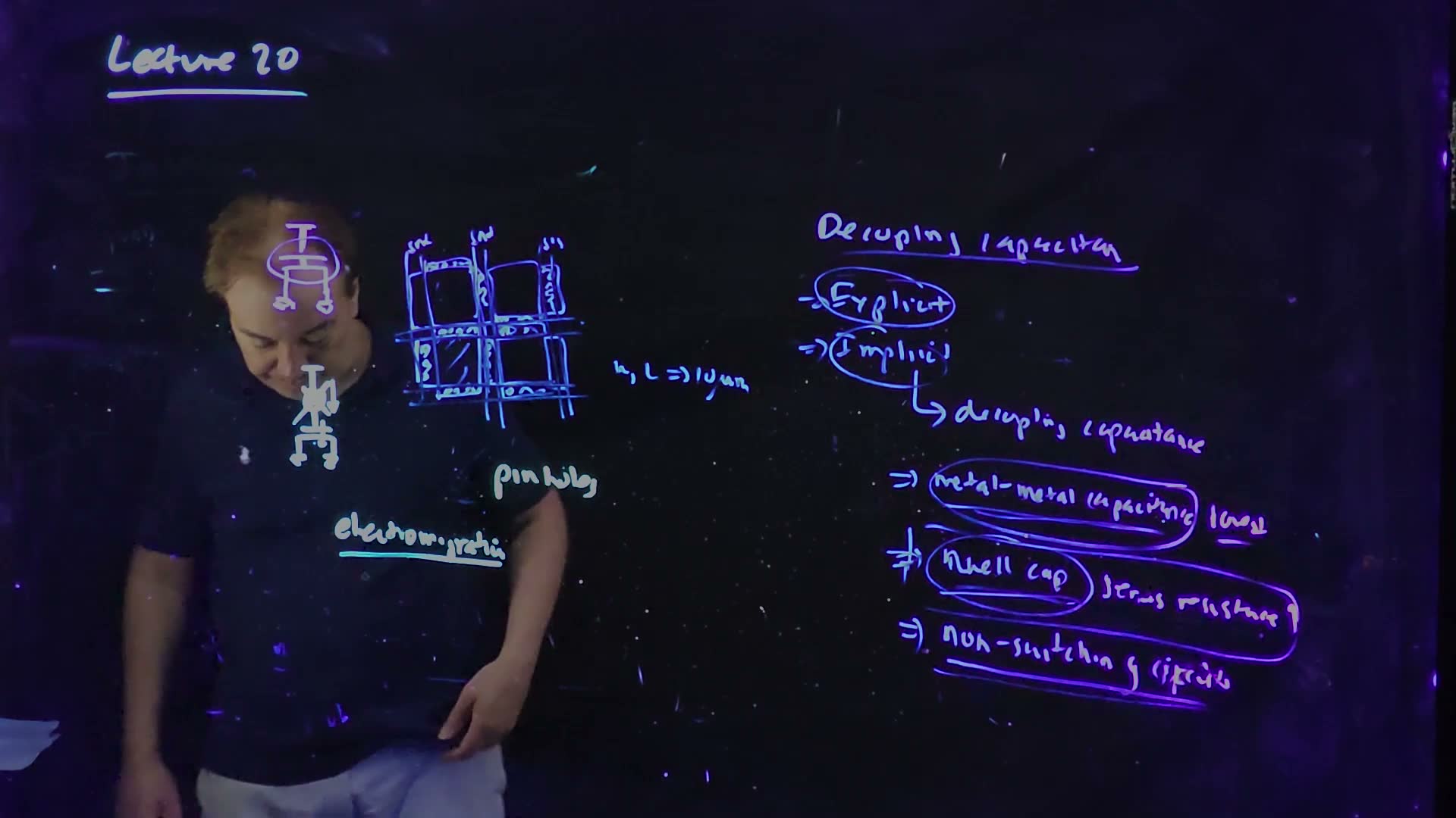
Fair copy of the board above (Lecture20 @ 72:10), mark for mark in its own layout. All black: the pale pen (the two devices, “pinholes” and “electromigration”), the blue pen (the tiling, “W, L ⇒ 10 µm”, the circles round “Explicit” and “Implicit” and the stroke through the arrow before “nwell cap”) and the violet pen (the circle round the top device and the long oval round the “nwell cap” line) mark the order of writing, not separate layers. The list at the right is the one from 64:23, in the same places as that copy. The rest of 64:23 was wiped after 65:57. The top device lies over the lecturer’s face in this frame; it is checked against 68:50, where it is clear. The tiling’s strokes are straightened and the writing is levelled.

Why small cells

Unit cells, not one big device (speech and board, 66:55–69:51)

1. The tempting design. One very large transistor, with a huge width and length, all of its area gate.
2. Why it fails. It has a large series resistance (67:05–68:07). With a long channel, the charge must travel far along the inverted channel to reach the source and drain contacts; with a very wide gate, it must travel far along the poly. Both put resistance in series with the capacitance, and a decap behind series resistance is slow (Section 11).
3. Why size is so costly added. The channel and the gate are each a distributed RC line: resistance and capacitance spread along them together. As Chapter 20 showed for wires, such a line’s time constant grows as the square of its length. Make the cell 10 times longer and its time constant grows 100 times.
4. The fix. Make a unit cell of moderate size, “typical width and length … something like 10 microns” board, and tile many of them, joined by metal: lower-metal straps to the sources and drains (ground), upper-metal straps to the poly (V_DD). The metal carries the current with little resistance; within each cell the charge travels at most a few microns.
5. Where it goes. Make a decap cell and drop it “wherever you have any white space in your design” (69:51).

Pinholes and fuses

A large area of thin oxide is likely to have defects (70:21–71:19). A pinhole, a short through the oxide, makes a cell a low-resistance path from $V_{DD}$ to ground, which “would obviously be devastating”. So technologies put a fuse in the decap cells: if a cell leaks too much, its fuse blows and the cell is taken out. These are electromigration fuses: they use on purpose the electromigration that designers otherwise avoid (Chapter 23, Lecture 22), so that a defect in one large-area decap does not cost the whole chip its yield.

A worked example

An added example added, by ratio.

One big device against unit cells

1. The same capacitance. Replace one decap device whose channel is 100 µm long by ten cells of 10 µm, strapped in metal: the same total gate area, so the same capacitance.
2. The time constant. Inside each cell the distance the charge travels is 10 times shorter. Both its resistance and its capacitance along that path scale with the length, so the time constant scales with the square: $10^2 =$ 100 times smaller.

Traps.

• The gate at ground. An NFET with its gate at ground and its source and drain at $V_{DD}$ has an off channel and far less capacitance; the gate must be at $V_{DD}$VDD​.
• One large rectangle “for density”. The area is the same, the series resistance is not.

Check yourself Why is the MOS decap an NFET with its gate at V_DD, rather than with its gate at ground?

With the gate at $V_{DD}$ and the source and drain at ground, $V_{GS} = V_{DD} > V_T$VT​: the channel is inverted, so the full oxide capacitance $C_{ox}WL$ sits between the supplies. With the gate at ground the channel is off and the capacitance is much smaller.

Check yourself A decap array uses 20 µm cells. Changing to 10 µm cells costs some area in extra contacts and straps. By what factor does each cell's time constant change, and why might the area be worth it?

The time constant scales as the square of the cell size: $(20/10)^2 = 4$ times smaller. A decap that responds four times faster can serve faster current edges, which is the decap’s whole job; a slower one, however large, only helps with slow fluctuations.

On the exam

The topics of this chapter appear in two of the four past finals (FN12 and FN17): 30 points that can be read, plus FN17-3c, whose point value is overwritten and illegible. FN10 and FN19 have none. No past part asks for repeaters, coupling noise or the Miller factor directly; the interconnect practice page, FW1 (Elmore wires, repeaters, clock-tree wires, power grids and decap), solves the parts below, adds variations on the rest, and this chapter solves none of them.

Part	Points	What it asks	Sections
FN17-1b	5	a decap target for a 1 nF clock load and at most 10% droop	§10
FN17-3b	11	the jitter a clock tree’s buffers get from supply noise of 10%, given their supply sensitivity	§8 (with Chapter 20 for the buffer delays of 3a)
FN17-3c	illegible	the same wires with an inductance per unit length: should inductance be included?	§7, §6
FN12-3	7	why grids are preferred for power and ground distribution (at least two reasons)	§9, §6
FN12-4	7	at least three sources of on-chip decap, and why on-chip decap is needed for supply integrity	§11, §12, §10

Notes for the practice page.

• FN17-3b needs FN17-3a’s buffer delays: the supply sensitivity applies to the silicon delay only, not to the tree’s wires (§8). Three points must be settled there from the paper: how much wire the tree has (the key counts 64 000 µm, the figure gives more), the load at the leaf (the key’s figure and its arithmetic disagree), and whether “10% supply noise” is a one-sided droop or ±10%, which doubles the edge’s range. Each changes the number, so this chapter gives none. The 1.2 V nominal supply is not needed: only the fraction enters.
• FN17-3c gives no slew time, so use §7’s step 5. The paper’s wires (0.1 Ω/µm, 0.2 fF/µm, 0.1 nH/mm) have $\ell^{*} = 0.447$ mm and $2\mathcal{L}/\mathcal{R} = 2$ ps. (a) The tree’s segments are 1000 to 4000 µm, all far beyond 0.447 mm, so every one is an RC line. (b) The stem’s $\tau_{inv} = 100$ ps means edges far slower than 2 ps. The key’s route, $\mathcal{R}/\mathcal{L} = 10^{12}$ rad/s against the signals’ frequency content, is the same test as (b).
• FN12-4’s key lists four sources and does not answer the “why”: answer it from §10 (a local charge reservoir, so the transient current does not pass through the package’s inductance).

Memorize.

• $h = \sqrt{R_{buf}C/(RC_{buf})}$ and $k = \sqrt{\tfrac12RC/(R_{buf}C_{buf})}$21​RC/(Rbuf​Cbuf​)​, with the totals $R$ and $C$C; $k$ is the square root of (intrinsic Elmore delay ÷ FO1 delay), and counts the driver.
• The worst coupling glitch, $\Delta V = V_{DD}\,C_c/(C_c + C_g)$Cg​); the Miller cases: same direction 0, quiet $C_c$Cc​, opposite $2C_c$2Cc​.
• $t_{RC} = \tfrac12\mathcal{R}\mathcal{C}\ell^2$21​RCℓ2, $t_{LC} = \sqrt{\mathcal{L}\mathcal{C}}\,\ell$LC​ℓ, against the slew time: C, then LC, then RC.
• Supply noise: DC = IR drop (resistance), AC = $L\,dI/dt$ (inductance).
• Grids: low R and low L through many parallel paths; built-in metal–metal decap; nearby returns for signals; the cost is routing.
• Decap sources: metal–metal (lowest series resistance), n-well, non-switching circuits (implicit); thin-oxide MOS decap, as unit cells of about 10 µm (explicit).

Derive (with the path).

• The repeater optimum. One segment’s three Elmore terms times $k$k; expand to $RC/(2k) + RhC_{buf} + R_{buf}C/h + kR_{buf}C_{buf}$kRbuf​Cbuf​; balance the $k$-pair and the $h$-pair; $T_{min} = (2 + \sqrt2)\sqrt{RC\,R_{buf}C_{buf}}$2​)RCRbuf​Cbuf​​; $\ell/k$ and $h$ do not depend on $\ell$ℓ.
• The inductance window. Equate $t_{RC}$ and $t_{LC}$tLC​: $\ell^{*} = 2\sqrt{\mathcal{L}\mathcal{C}}/(\mathcal{R}\mathcal{C})$2LC​/(RC), where both are $2\mathcal{L}/\mathcal{R}$2L/R; inductance matters only if $t_{slew} \lesssim 2\mathcal{L}/\mathcal{R}$2L/R.
• A supply-induced delay change. $\Delta\tau \approx S\,\tau_{silicon}\,\Delta V_{DD}/V_{DD}$Sτsilicon​ΔVDD​/VDD​, gates only; varying from cycle to cycle, it is jitter.
• The decap target. Conserve the decap’s charge across one edge: $\Delta V/V_{DD} = C_{sw}/(C_{sw} + C_{decap})$Cdecap​), so $C_{decap} \ge C_{sw}(1 - \varepsilon)/\varepsilon$ε)/ε.

Method cards. The playbook’s cards for these families, when it exists: repeater sizing; coupling noise and the Miller factor; the inductance window; supply noise and decap.

The lecture’s boards

The boards of Lecture 20 used in this chapter (22 frames)

Lecture20 @ 01:37 Interconnect: C, R ⇒ RC delay; L; widen the wires; repeater insertion

Lecture20 @ 09:33 h and k, before the ½ is moved into the numerator

Lecture20 @ 11:59 the repeater model, T_delay, h and the boxed k; 1 mm

Lecture20 @ 14:12 a wire in cross-section with its neighbours

Lecture20 @ 15:35 floating/coupling caps and ground caps

Lecture20 @ 18:25 coupling noise: the victim dips as the aggressor falls

Lecture20 @ 19:55 ΔV = V_DD C_c/(C_c + C_g)

Lecture20 @ 22:33 weak driver, long wire, pass-transistor latch storing 1/0

Lecture20 @ 23:48 the latch flipped to 0/1 with clk = 0

Lecture20 @ 25:06 repeaters on the victim wire as a fix

Lecture20 @ 30:30 noise on delay: the superposition

Lecture20 @ 31:57 the delayed, stepped victim waveform

Lecture20 @ 39:54 the current loop: V = L dI/dt, R + jωL

Lecture20 @ 42:57 RC, LC and the slew time in the half-micron world

Lecture20 @ 44:32 scaling: the slew time falls, the RC curve moves

Lecture20 @ 49:37 C, transmission line, RC

Lecture20 @ 55:29 supply noise: dc IR drop, ac L dI/dt; the grid

Lecture20 @ 57:57 bond-wire inductance and decoupling capacitance

Lecture20 @ 61:44 implicit decap: metal–metal and the n-well

Lecture20 @ 64:23 the decap sources and their series resistance

Lecture20 @ 68:50 the MOS decap and its first unit cells

Lecture20 @ 72:10 unit cells, W, L ≈ 10 µm, pinholes, electromigration fuses