20. Wires: resistance, capacitance and Elmore delay

So far the course has drawn wires as perfect connections: one node, one voltage, no delay. Lecture 19 turns to the back end of the line, the metal wires above the transistors, and asks what they add to a circuit. They add capacitance almost always, resistance sometimes, and inductance occasionally. The chapter works out a wire’s resistance and capacitance from its shape, shows why shrinking a technology makes long wires slower while the transistors get faster, and builds the course’s one tool for the delay of a resistive wire: the Elmore delay, a single number in picoseconds. With it the chapter answers when a wire’s resistance matters, handles wires that branch to several receivers, works the lecture’s own 1 mm example (104.5 ps), and compares the cures: widening the wire, breaking it with repeaters, and tapering it.

After this chapter you can:

1. compute a wire’s resistance from its sheet resistance and its number of squares, and its capacitance from 0.1 fF/µm or from an areal-plus-fringe formula;
2. say how a wire’s R, C and RC change when the wires shrink but the chip does not;
3. write the Elmore delay of any RC ladder or tree to a chosen receiver, and split it into its intrinsic and extrinsic parts;
4. derive the ½ in $\tfrac12\mathcal{R}\mathcal{C}L^2$ and use the uniform-line formula with a load;
5. decide whether a wire’s resistance matters by comparing its Elmore delay with the slew of the edges it carries;
6. compute what widening or tapering a wire does to its delay, and say when each helps;
7. explain why repeaters turn the delay’s $L^2$ growth into roughly linear growth (how many and how big is Chapter 21’s question).

Boxes and equations marked board were written in the lecture. Parts marked added are explanations or examples this guide adds.

Symbols

Symbol	Meaning	Unit	First appears
$\rho$	bulk resistivity of the metal	Ω·cm	§1
$t$	thickness of a wire (its metal layer)	µm	§1
$W$	width of a wire	µm	§1
$L$	length of a wire (Chapter 21 writes this length $\ell$ℓ, because its $L$ is inductance)	µm, mm	§1
$A$	cross-sectional area of a wire, $tW$ (in §2 also the facing area of two wires)	µm², cm²	§1
$R_\square$	sheet resistance, $\rho/t$ρ/t, in ohms per square (the board says “sheet resistivity”; symbol added)	Ω/□	§1
$L/W$	the number of squares in a wire	—	§1
$\mathcal{R}$	resistance per unit length, $R_\square/W$ (the board’s script R)	Ω/µm	§1
$\mathcal{C}$	capacitance per unit length (the board’s script C)	fF/µm	§1
$C_w$	the whole wire’s capacitance, $\mathcal{C}L$	fF	§1
$s$	the scaling factor: dimensions shrink by $1/s$ (Chapter 4 writes κ)	—	§2
$s_L$	the factor by which wire lengths scale	—	§2
$d$	the gap between two neighbouring wires (the board writes $t$ there; symbol added)	µm	§2
$R_i$Ri​, $C_i$	the resistors and capacitors of an extracted RC network, numbered from the driver as on the board	Ω, fF	§3
$C_{load}$	the receiver’s input capacitance at the end of a wire	fF	§3
$T_{Elmore}$	the Elmore delay (the board writes $T_{elmore}$Telmore​)	ps	§3
$\tau$	the time constant of one RC (one pole)	ps	§3
$t_r$	the slew: how long an edge takes to switch (the lecturer’s “slew rate”; symbol added)	ps	§6
$C_{near}$Cnear​, $R$R, $C_{far}$	the π model of a wire as its driver sees it	fF, Ω	§6
$\tau_{inv}$	the fan-out-of-one (FO1) delay of an inverter (Chapter 7)	ps	§6
$R_k$Rk​, $C_k$	resistance and capacitance of segment $k$ of a path added	Ω, fF	§7
$C_{down,k}$	all the capacitance beyond the far end of path segment $k$k, side branches included added	fF	§7
$x$x, $dx$	distance along a wire from its driver, and a short slice there	µm	§4
$r(x)$	the resistance between the driver and the point $x$x, $\mathcal{R}x$	Ω	§4
$k$	the number of equal sections (§4) or repeater pieces (§9) a wire is cut into	—	§4
$L_p$	the length of one piece between repeaters	mm	§9
$C_{in}$	a gate’s input capacitance (Chapter 7)	fF	§7
$R_{shared}(c, B)$	the resistance that capacitance $c$‘s path to the driver shares with the path to receiver B added	Ω	§7
$C_{side}$	a side branch’s capacitance, lumped where it leaves the path	fF	§7
$C_{XC}$	the wire capacitance of the branch from X to C in §7’s example	fF	§7
$C_{areal}$	capacitance per unit area under a wire (the board’s “areal”)	fF/µm²	§8
$C_{fringe}$	fringing capacitance per unit length from a wire’s sides	fF/µm	§8
$T(W)$T(W), $T$	the Elmore delay as a function of the width (§8), and of a tapered wire (§10)	ps	§8

1. Wire capacitance and resistance

You need

Resistance of a bar added (from circuits). A bar of a material with resistivity $\rho$ρ, length $L$ along the current and cross-section $A$ has resistance $R = \rho L/A$ρL/A: longer is worse, fatter is better.

Wire capacitance (Chapter 5, from Lecture 5’s board). A minimum-width wire has about 0.1 fF of capacitance per µm of length. It is a load like any other: the gate that drives the wire must charge it.

Gate capacitance (Chapter 7). A transistor gate has a capacitance per µm of width; the past finals use 1–2 fF/µm. So a wire’s capacitance can be quoted as the width of gate it is equivalent to.

The question. A wire is a strip of metal with a length, a width and a thickness. What does it add to the circuit, and how big is each part?

What a wire adds (board, 00:33–07:37)

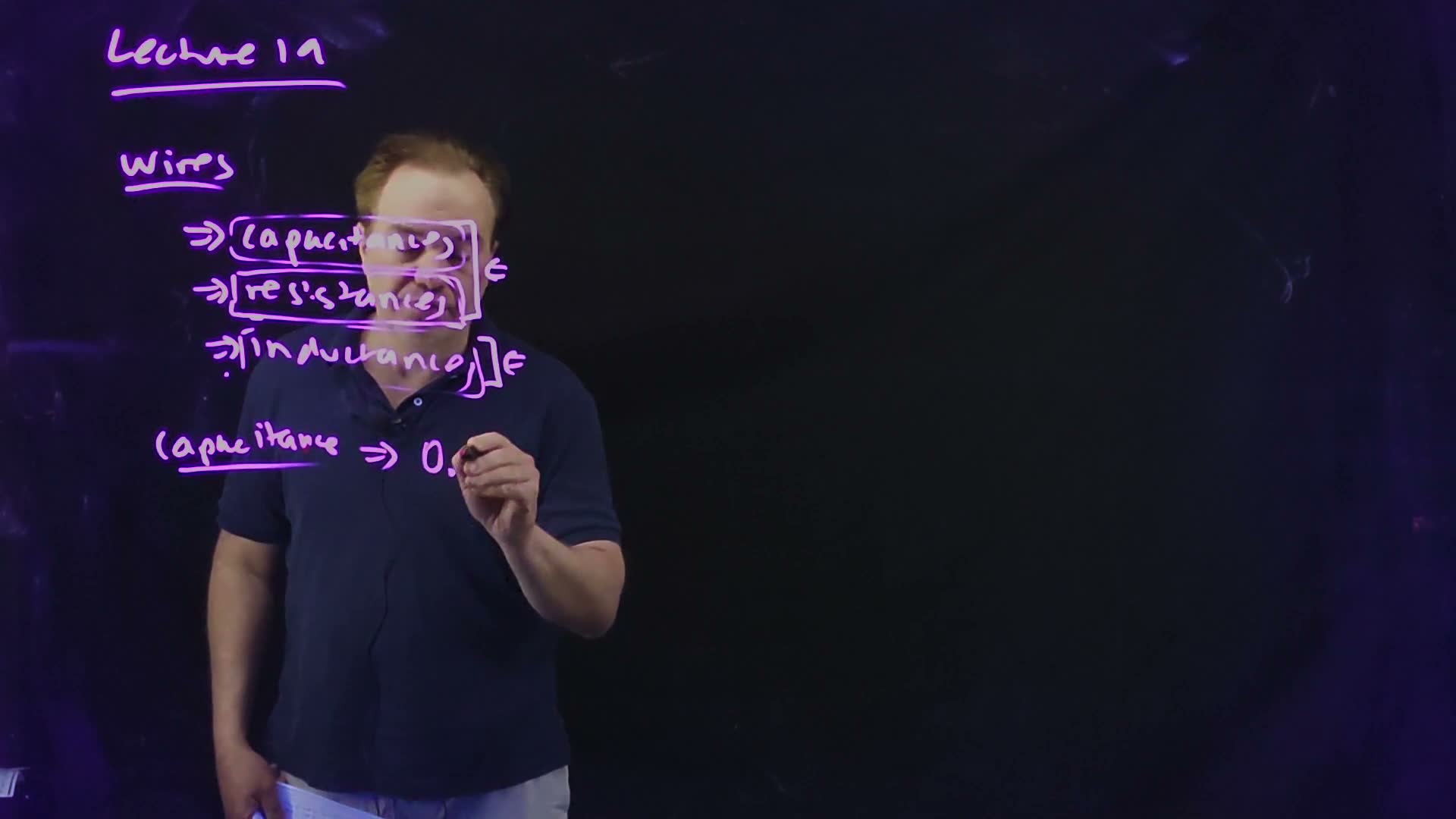
1. Three parasitics, in order of how often they matter. Wires add capacitance, resistance and, in some cases, inductance board. “The capacitance of the line will matter for … nearly all cases … In other cases, we’ll have to worry about the resistance in addition to the capacitance … and in other cases … the inductance” (01:04–01:35). This chapter does the first two; inductance is Chapter 21’s. For capacitance the board gives the rule of thumb 0.1 fF/µm, marked “ROM”, a rough order of magnitude: the real value depends on the wire’s neighbours (01:35–02:04) board. It is the same value Lecture 5 gave.
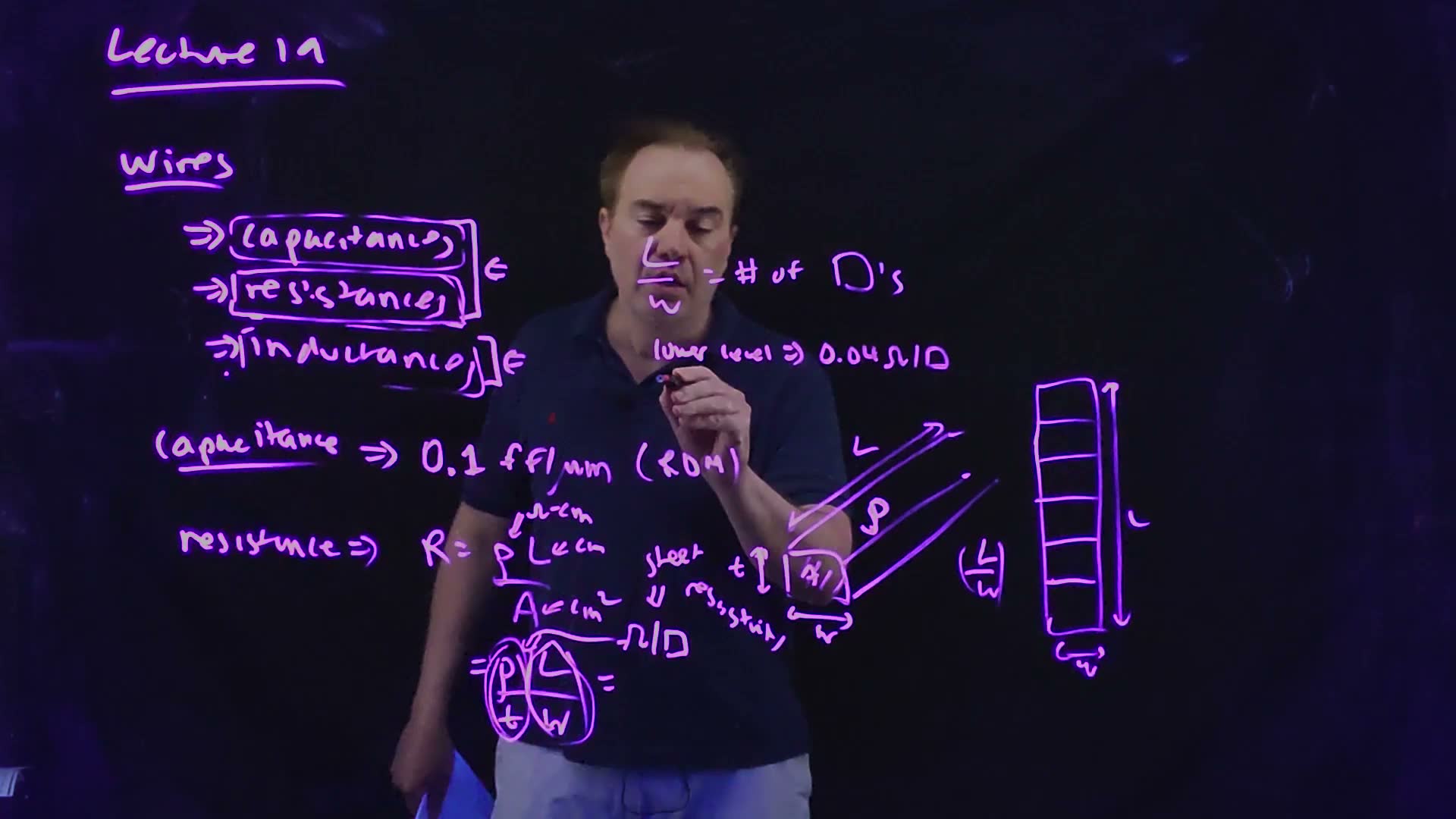
2. Resistance from the shape. For a wire of resistivity $\rho$ (in Ω·cm), length $L$ and cross-section $A$A, $R = \rho L/A$ board. Write the cross-section as thickness times width, $A = tW$tW, and split the expression in two (02:44–03:42): $R = \frac{\rho}{t}\cdot\frac{L}{W}.$ The first factor depends only on the metal layer: its material and its thickness. It is called the sheet resistance, $R_\square$ (the board says “sheet resistivity”), and is quoted in ohms per square, Ω/□.
3. Squares. The second factor, $L/W$L/W, is a pure number: cut the wire along its length into squares of side $W$W, and there are $L/W$ of them (04:00) board. Every square has the same resistance, $R_\square$R□​, whatever its size, because a square twice as long is also twice as wide. So $R = R_\square \cdot (L/W)$(L/W), “ohms per square” times the number of squares. The process fixes the thickness of each layer, so $R_\square$ is a number the technology gives you; the designer controls only $L$ and $W$ (04:33).
4. Numbers, and why copper. Lower metal levels have about 0.04 Ω/□ board. Upper levels are thicker, so their sheet resistance is lower (05:00–05:25); the board writes the upper range as “0.01–0.2† Ω/□”. † The 0.2 is a slip: read the range as 0.01–0.02 Ω/□ added, because a thicker layer of the same metal cannot have five times the 0.04 Ω/□ of a thinner one, and the lecturer says the number “will drop”. That upper end is this guide’s inference; the direction, below 0.04, is the lecture’s. Until the 0.13 µm node interconnect was aluminum; from 130 nm on it is copper, because copper’s resistivity is lower (05:51). Copper must not reach the silicon, so every copper wire sits in a thin liner of a refractory metal, a diffusion barrier (06:46).

A wire’s resistance, redrawn from the board (Lecture19 @ 05:15, 07:37). Left: a bar of resistivity $\rho$ρ, length $L$L, width $W$ and thickness $t$t, so $R = \rho L/(tW)$ρL/(tW). Right: seen from above, the same wire is $L/W$ squares of side $W$ in a row (seven here). Each square has the sheet resistance $R_\square = \rho/t$ρ/t, so $R = R_\square \cdot L/W$L/W.

The board (Lecture19 @ 07:37)

Lecture19 @ 07:37The first board: the three parasitics, 0.1 fF/µm, R = (ρ/t)(L/W), sheet resistance and squares, the two levels' values (the upper range's 0.2 is a slip for 0.02) and copper with its liner.

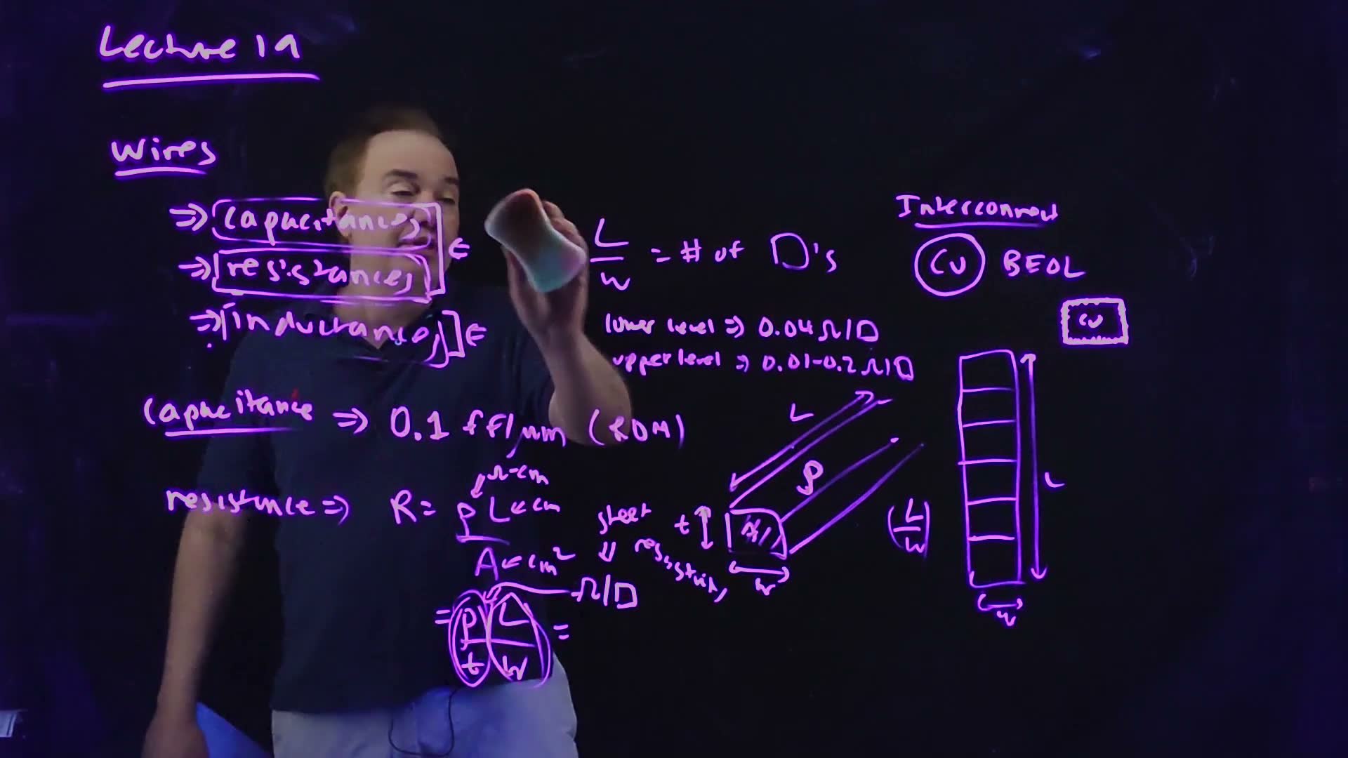
Fair copy of the board above (Lecture19 @ 07:37), mark for mark in its own layout. The board is in one pen (violet), copied in black. The arrows after the bracket and after “inductance” are set as ⇐. † The upper level’s range reads 0.01–0.2 Ω/□ on the board: the 0.2 is a slip for 0.02, since the thicker upper levels have a lower sheet resistance than the lower level’s 0.04 Ω/□. The grey band inside the boxed Cu is the liner round the copper. The lecturer’s body and hand cross the list and “0.1 fF/µm” in this frame, but the ink shows through, so nothing is restored. The writing is levelled; “resistivity” keeps its slant, as there is no room to set it level.

The wiring levels added (a sketch; the lecture names lower and upper levels at Lecture19 @ 05:00–05:25 and draws the boxed copper at 07:37). Upper levels are thicker, so their sheet resistance $R_\square = \rho/t$ is lower. Each copper core (blue) sits in a thin liner (orange), a refractory-metal diffusion barrier that keeps the copper out of the silicon; the wires sit in dielectric over the silicon.

Wire resistanceboard

$$R = \rho\,\frac{L}{A} = \frac{\rho}{t}\cdot\frac{L}{W} = R_\square\,\frac{L}{W}$$

Holds when: a uniform rectangular wire with the current along its length; contacts, vias and corners are not included

Per unit length this is $\mathcal{R} = R_\square/W$ (Ω/µm), so a wire of length $L$ has $R = \mathcal{R}L$RL. The board writes $\mathcal{R}$ and $\mathcal{C}$ (script letters) for the per-length values from its Elmore board on; this chapter does the same.

Wire capacitance, rule of thumbboard

$$C_w \approx \mathcal{C}L, \qquad \mathcal{C} \approx 0.1\ \text{fF}/\mu\text{m}$$

Holds when: an average minimum-width wire; an order-of-magnitude estimate, not an extraction (Section 8 gives the width-dependent form)

Memorize or derive. Memorize $R = R_\square L/W$ and 0.1 fF/µm. $\mathcal{R} = R_\square/W$ follows in one line.

A worked example added. A wire 1 mm long and 0.4 µm wide, the size of the lecture’s example in Section 5.

Resistance and capacitance of a 1 mm wire

1. Count the squares. $L/W = 1000/0.4 = 2500$ squares.
2. Resistance on a 0.04 Ω/□ layer. $R = 0.04 \times 2500 = 100\ \Omega$100 Ω. On a 0.076 Ω/□ layer, the value the lecture’s example uses, $R = 0.076 \times 2500 = 190\ \Omega$190 Ω.
3. Capacitance. $C_w = 0.1 \times 1000 = 100$ fF. At 2 fF per µm of gate width that is the load of 50 µm of gate: a wire 1 mm long loads its driver like a large gate.

Traps.

• Multiplying $R_\square$ by $W/L$W/L, or by an area. It is the number of squares, $L/W$L/W. A wider wire has fewer squares and less resistance.
• Reading Ω/□ as a different unit from Ω. A square is dimensionless; “per square” just says what to multiply by.
• Using a lower level’s sheet resistance for a thick upper-level wire. The metal is the same, but the thickness is not.

Check yourself A wire 2 mm long and 1 µm wide runs on a 0.02 Ω/□ layer. What is its resistance?

$L/W = 2000/1 = 2000$ squares, so $R = 0.02 \times 2000 = 40\ \Omega$40 Ω.

Check yourself The same wire at 0.1 fF/µm: what is its capacitance, and how many µm of gate (at 2 fF/µm) does it equal?

$C_w = 0.1 \times 2000 = 200$ fF. At 2 fF/µm that is $200/2 = 100$ µm of gate width.

Check yourself The upper metal levels are the same copper as the lower ones. Why is their sheet resistance lower?

They are thicker. $R_\square = \rho/t$ρ/t: the same $\rho$ over a larger $t$t.

2. Scaling wires: why RC gets worse

You need

Constant-field scaling (Chapter 4). Shrink every dimension and voltage of a transistor by a factor κ (this lecture writes $s$s): a gate’s delay $CV/I$ falls as $1/s$1/s. Transistors get faster.

Parallel-plate capacitance added (from circuits). Two conductors facing each other over a gap have a capacitance proportional to their facing area divided by the gap.

Wire resistance (Section 1). $R = \rho L/A$ρL/A, with $A = tW$ the wire’s cross-section.

A wire’s resistance (Lecture19 @ 05:15, redrawn): $R = \rho L/(tW) = R_\square L/W$R□​L/W. Original figure ↑

The question. Transistors shrink every technology generation and get faster. The wires shrink with them. What happens to a wire’s resistance, its capacitance and their product, which Section 3 will show sets its delay?

Scaling a wire (board, 08:28–13:45)

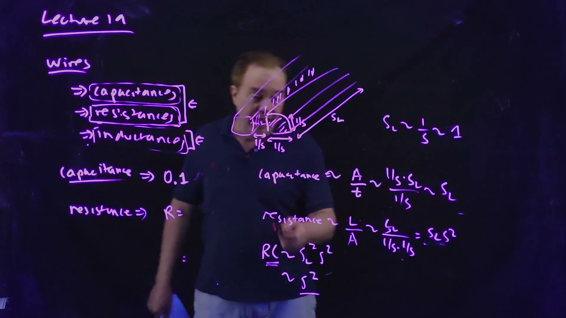
1. What shrinks, and what doesn’t. Picture three neighbouring wires. Scale each wire’s thickness and width, and the spacing between wires, by $1/s$1/s, just as the transistors are scaled board. Their length gets its own factor $s_L$sL​, because “we don’t make our chips smaller … we just put more transistors on there” (09:29): a wire that crosses the chip keeps its length, so for such a wire $s_L \approx 1$1.
2. Capacitance. The capacitance between two neighbours is a parallel plate: the facing side area over the gap $d$ between them (the board writes $t$ for this gap). The facing area is thickness times length, $\sim (1/s)\cdot s_L$sL​; the gap is $\sim 1/s$1/s. So $C \sim \dfrac{(1/s)\,s_L}{1/s} = s_L$ board: for a wire that keeps its length, the capacitance does not change. That is why 0.1 fF/µm has held for many generations.
3. Resistance and RC. The resistance is length over cross-section: $R \sim \dfrac{s_L}{(1/s)(1/s)} = s_L s^2$ board. The product is $RC \sim s_L^2 s^2$sL2​s2. If wire lengths shrank with everything else, $s_L = 1/s$1/s, the RC would stay the same. But $s_L \approx 1$1, so $RC \sim s^2$ (circled on the board): it grows as the square of the scaling factor.
4. Wires against gates added. A gate’s delay falls as $1/s$ (Chapter 4) while a long wire’s RC grows as $s^2$s2, so relative to the gates the wire gets worse as $s^3$s3. “The transistors are getting faster and the wires are getting slower” (12:26). When this lecture was recorded, the lecturer recalled that “in quarter micron or half micron technology, you didn’t really worry much about the RC delays of the line”; now many wires need repeaters (Section 9), and repeaters “wind up being a not insignificant amount of the power that’s being dissipated in a modern microprocessor” (12:52).

Wire scaling, redrawn from the board (Lecture19 @ 13:45). Thickness, width and spacing shrink by $1/s$1/s; the length scales by $s_L$sL​, about 1 for a wire that crosses the chip. The capacitance between neighbours is set by the facing area over the gap (hatched on the left wire’s face toward the gap), so it scales as $s_L$sL​; the resistance as $s_L s^2$sL​s2.

The board (Lecture19 @ 13:45)

Lecture19 @ 13:45The scaling board: C ∼ s_L, R ∼ s_L s², RC ∼ s_L² s² ∼ s² for wires whose length does not scale. The board's t in A/t is the gap between the wires.

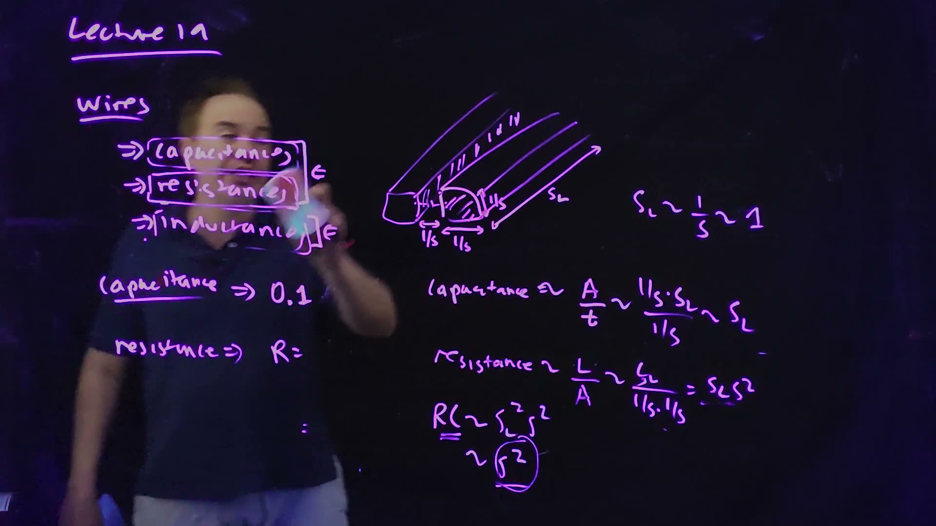
Fair copy of the board above (Lecture19 @ 13:45), mark for mark in its own layout. One pen (violet), copied in black. At the left stands what is left of the first board: the list as at 07:37, and of its lower lines only “capacitance ⇒ 0.1” and “resistance ⇒ R =”; the rest was erased. The lecturer’s hand covers the right ends of the bracket and of the inductance brackets in this frame; they are copied from 08:28. At the right, two wires side by side: the gap, the width and the thickness each scale as $1/s$ and the length as $s_L$sL​; the short strokes between the wires mark the field of their coupling capacitance. The scaling lines are levelled.

Relative delays as the technology scales by $s$ added, computed from $RC \sim s_L^2 s^2$ and Chapter 4’s gate delay $\propto 1/s$1/s. A long wire ($s_L = 1$sL​=1) grows as $s^2$s2; a local wire whose length shrinks with the logic ($s_L = 1/s$sL​=1/s) stays the same; a gate’s delay falls as $1/s$1/s. At $s = 2$ the long wire is 4 times slower and the gate twice as fast.

Wire scalingboard

$$C \sim s_L, \qquad R \sim s_L\,s^2, \qquad RC \sim s_L^2\,s^2$$

Holds when: thickness, width and spacing all scale by 1/s; the length by s_L (about 1 for a wire that crosses the chip, 1/s for a local wire that shrinks with its logic)

Memorize or derive. Derive it in three lines: capacitance is (thickness × length)/gap, resistance is length/(thickness × width), multiply.

A worked example added. One technology node shrinks dimensions by about 0.7, so $s = \sqrt2$ (Chapter 1’s node ladder).

One node and two nodes of scaling

1. One node, $s = \sqrt2$2​. A long wire’s RC grows by $s^2 = 2$2. A gate’s delay falls to $1/\sqrt2 = 0.707$ of what it was. Relative to the gates, the wire is $2/0.707 = 2.83$ times slower.
2. Two nodes, $s = 2$2. The wire’s RC grows by 4, the gate’s delay falls to 0.5, and the ratio worsens by 8, which is $s^3$s3.

Traps.

• Scaling a global wire’s length by $1/s$1/s. Only local wires, inside a block that shrinks, get shorter. A wire across the chip keeps its length.
• Expecting the capacitance per length to grow. It stays about the same; it is the resistance per length that grows, as $s^2$s2.

Check yourself Inside a block, the wires shrink in length with the logic (s_L = 1/s). How does their RC change?

$RC \sim s_L^2 s^2 = (1/s)^2 s^2 = 1$1: it does not change.

Check yourself Over three nodes, s = 2√2. By what factor does a global wire's RC grow, and by what factor does it grow relative to a gate's delay?

$s^2 = 8$8, so the RC grows 8 times. The gate’s delay falls to $1/s = 0.354$0.354, so relative to the gates the wire is $s^3 = 22.6$ times slower.

3. The Elmore delay of an RC ladder

You need

One RC added (from circuits). A step through a resistor $R$ into a grounded capacitor $C$ gives $v(t) = 1 - e^{-t/RC}$ of the step: one pole, with time constant $\tau = RC$RC. It reaches 50% at $\tau\ln 2 = 0.69\tau$0.69τ, and goes from 10% to 90% in $\tau\ln 9 = 2.2\tau$2.2τ.

The course’s delay convention (Chapter 7). Gate delays are quoted as a resistance times a capacitance, $t = (R/W)\,C_{load}$(R/W)Cload​, with the resistance fitted so that this product is the delay; nobody multiplies by ln 2 again. The Elmore delay below is quoted the same way, as the delay itself. Units: 1 kΩ × 1 fF = 1 ps, so 1 Ω × 1 fF = 0.001 ps.

Wire R and C (Section 1). $R = R_\square L/W$R□​L/W; about 0.1 fF of capacitance per µm.

The question. A wire has resistance and capacitance spread along its whole length. When a driver switches, how long does the far end take to follow?

The wire as an RC ladder

From a wire to a number (board, 15:39–19:40)

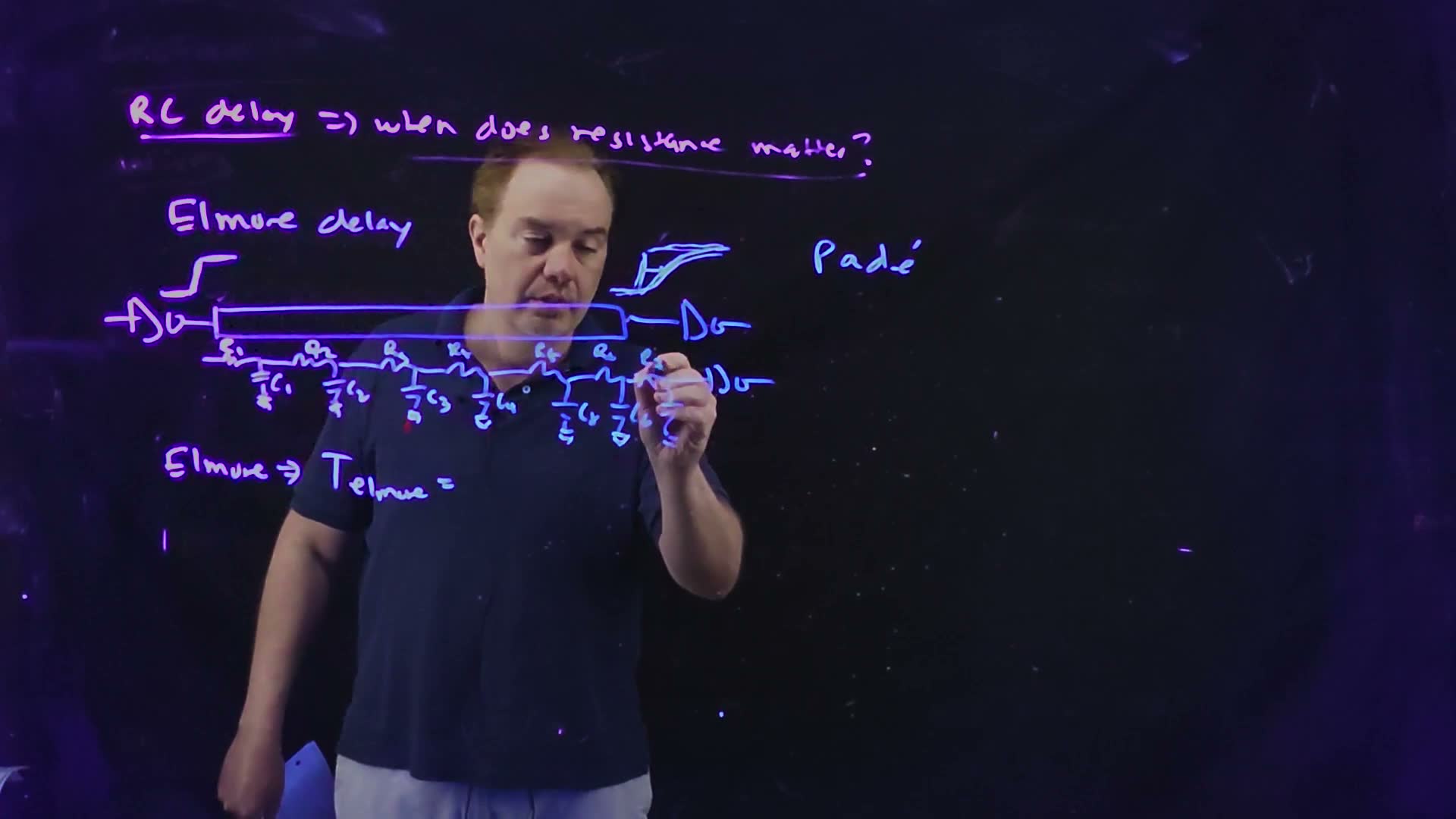
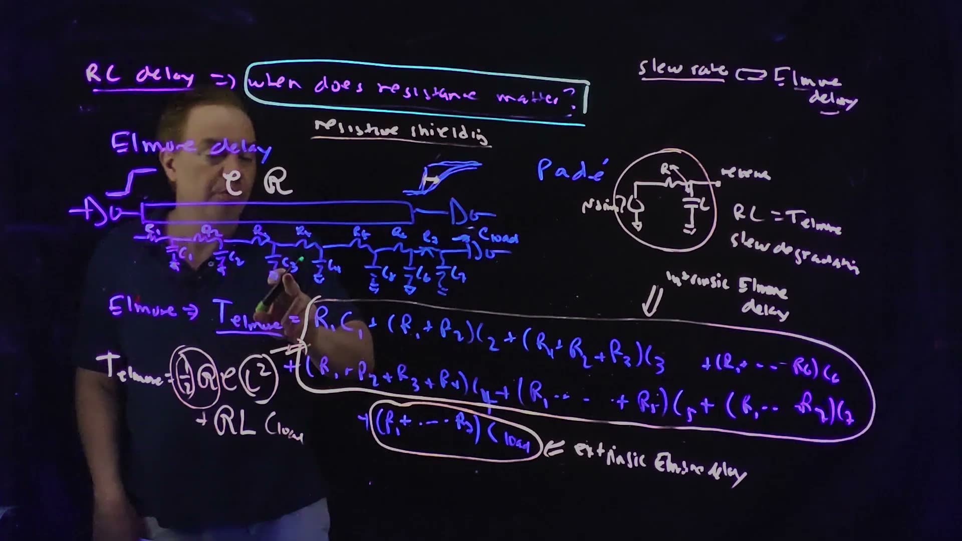
1. Extraction. An inverter drives a wire into another inverter. The layout tool (in the course, Calibre) can extract the wire into a network of resistors and capacitors: cut it into pieces, give each piece its resistance and its capacitance (16:00–16:49) board. The capacitors here go to ground. Capacitance to a neighbouring wire that is itself switching (a “floating cap”) is Chapter 21’s.
2. Why not always extract R? “Going in and extracting resistance everywhere … is going to really slow your simulations down” (14:20). So a designer needs to know when the resistance matters (Section 6 answers), and how big a delay to expect, to sanity-check the tools.
3. What the network does. It is a low-pass filter. The driver’s sharp edge arrives at the receiver later and slower (17:57–18:40). The board’s network has seven capacitors, so it is a seven-pole filter.
4. One pole instead of seven. The Elmore delay approximates the whole network by a single pole, a Padé approximation (the board writes “Padé”), and $T_{Elmore}$ is that pole’s time constant (19:14) board. The lecturer does not prove the formula; it comes next.

A wire and its extracted RC ladder, redrawn from the board (Lecture19 @ 24:23). The driver’s sharp edge arrives at the receiver later and slower. The ladder has seven sections, $R_1, C_1$ to $R_7, C_7$R7​,C7​, numbered from the driver; $C_{load}$ is the receiver’s input capacitance.

The board (Lecture19 @ 24:23)

Lecture19 @ 24:23The Elmore sum for the seven-section ladder, with its intrinsic and extrinsic parts looped in pink. The C₆ term was forgotten and added at the end of the first line.

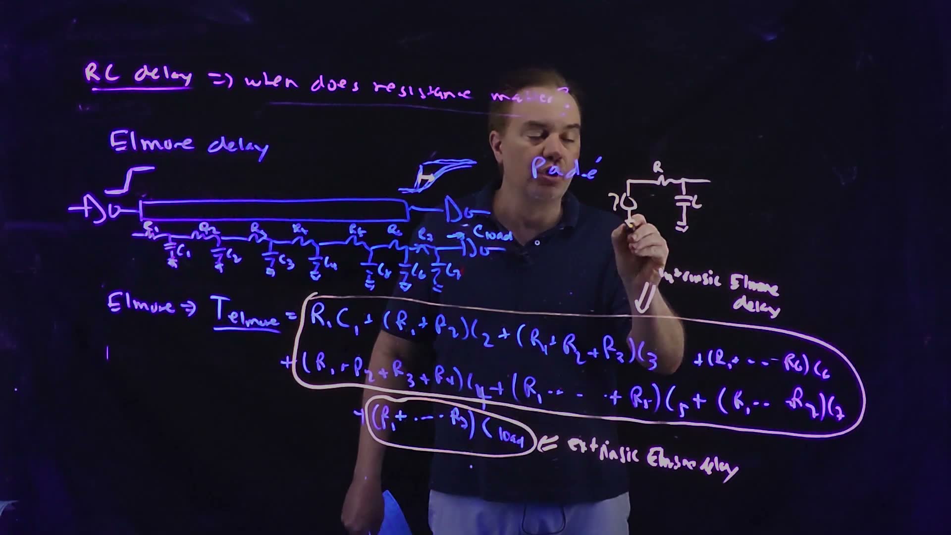
Fair copy of the board above (Lecture19 @ 24:23), mark for mark in its own layout. Black is the blue pen (the wire sketch, the ladder, “Padé” and the Elmore sum) and the violet pen (the title line). Magenta is the pale pink pen: the arrow between the receiver’s step and its slower edge, the two loops, the double arrow, “intrinsic Elmore delay” and “extrinsic Elmore delay”, and the small R–C circuit at the right. The $C_6$ term was forgotten and squeezed in, a little smaller, at the end of the first line. The lecturer’s head hides “matter?”, the end of its underline and part of “Padé” in this frame; they are copied from 23:38 and 24:39. His hand covers the start of “intrinsic” (copied from 23:38) and the source’s lower lead, which he is drawing: its ground appears at 24:39. The writing is levelled; the board’s lines drift down to the right.

The rule: each capacitor times its resistance back to the driver

The rule fits in one sentence: every capacitor counts with the resistance between it and the driver, the resistance its charging current must flow through (20:42–22:14) board. For the board’s ladder,

$$\begin{aligned} T_{Elmore} = {} & R_1C_1 + (R_1{+}R_2)C_2 + (R_1{+}R_2{+}R_3)C_3 + \dots \\ & + (R_1{+}\dots{+}R_7)C_7 + (R_1{+}\dots{+}R_7)\,C_{load}. \end{aligned}$$

$C_1$ charges through $R_1$ only. $C_3$ charges through $R_1$R1​, $R_2$ and $R_3$R3​. The receiver’s $C_{load}$Cload​, at the far end, charges through all seven.

The Elmore rule on a three-section ladder added. $C_2$C2​’s charging current flows through $R_1$ and $R_2$ (thick), so $C_2$ counts with $R_1 + R_2$R2​. Under each capacitor: the resistance it sees back to the driver. Values: $R_i = 100\ \Omega$100 Ω, $C_i = 20$ fF, $C_{load} = 50$ fF.

The terms split into two kinds (22:52–23:45) board:

• the intrinsic Elmore delay, every $C_i$ term: the wire’s resistance working against the wire’s own capacitance;
• the extrinsic Elmore delay, the $C_{load}$ term: the wire’s resistance working against the load. It “has nothing to do with the capacitance of the wire”.

They respond to different cures (Section 8), so it pays to keep them apart.

Elmore delay of an RC ladderboard

$$T_{Elmore} = \sum_{i} C_i \Big(\sum_{j \le i} R_j\Big) \;+\; C_{load}\sum_{j} R_j$$

Holds when: every capacitor is grounded; the driver switches with a step-like edge; a single-pole estimate, quoted as the delay itself

The receiver’s waveform

One number cannot be a waveform, but one pole can make one. Model the receiver’s waveform as the driver’s waveform passed through a single RC whose product is $T_{Elmore}$ (24:20–25:08) board. Only the product matters: “you can set R to one ohm, it doesn’t matter.” The board’s small circuit says it: a source with the driver’s waveform, one $R$R, one $C$C, the receiver, and “RC = $T_{elmore}$Telmore​”.

The single-pole model of the receiver, redrawn from the board (Lecture19 @ 24:39, 27:59). The source carries the driver’s waveform; the receiver sees it through one RC with $RC = T_{Elmore}$TElmore​.

The board (Lecture19 @ 24:39)

Lecture19 @ 24:39The single-pole model: the driver's waveform through one RC equal to the Elmore delay.

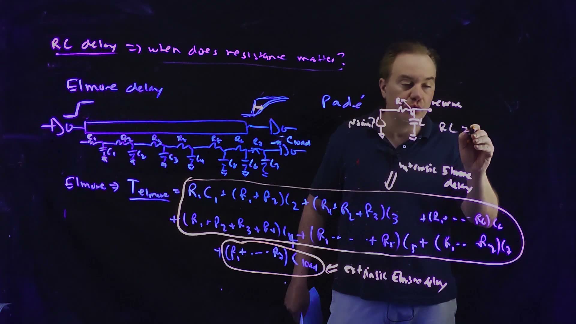
Fair copy of the board above (Lecture19 @ 24:39), mark for mark in its own layout. Black is the blue pen (the wire sketch, the ladder, “Padé” and the Elmore sum) and the violet pen (the title line). Magenta is the pale pink pen: the arrow at the receiver’s edge, the two loops, the double arrow, “intrinsic Elmore delay” and “extrinsic Elmore delay”, and the single-pole circuit at the right. Since 24:23 that circuit has gained “driver?” at its source, the source’s ground, an arrow at $R$R, a dot at the output node, “receiver” and "$RC =$", which the lecturer is still writing: it becomes $RC = T_{elmore}$Telmore​. The writing is levelled; the board’s lines drift down to the right.

From that one pole come the lecture’s two rules of thumb (25:10): the delay is about $T_{Elmore}$TElmore​, and the slew degradation (how much slower the edge gets) is about $2T_{Elmore}$2TElmore​, “again, order of magnitude”. The single pole of the You need fold says where these come from added: a step through $\tau$ crosses 50% at $0.69\tau$ and takes $2.2\tau$ from 10% to 90%. Those factors, 0.69 and 2.2, are of order one, so “delay ≈ $T_{Elmore}$TElmore​” and “slew ≈ $2T_{Elmore}$2TElmore​” are the same statements rounded, and the course quotes $T_{Elmore}$ itself. For a slow edge the delay is in fact almost exactly $\tau$τ: Section 6’s 300 ps edge through a 104.5 ps pole comes out 94.4 ps late.

What the Elmore delay predictsboard

$$\text{delay} \approx T_{Elmore}, \qquad \text{slew degradation} \approx 2\,T_{Elmore}$$

Holds when: order of magnitude; the receiver's waveform is the driver's through one pole τ = T_Elmore

Memorize or derive. Memorize the rule (the course does not derive it) and the two rules of thumb.

A worked example

An added example added, the three-section ladder of the figure: $R_1 = R_2 = R_3 = 100\ \Omega$100 Ω, $C_1 = C_2 = C_3 = 20$ fF, $C_{load} = 50$ fF.

The three-section ladder: $R_i = 100\ \Omega$100 Ω, $C_i = 20$ fF, $C_{load} = 50$ fF. Original figure ↑

The Elmore delay of three sections

1. The unit. $100\ \Omega \times 20\ \text{fF} = 2000\ \Omega\cdot\text{fF} = 2$ ps.
2. Intrinsic. $C_1$ sees 100 Ω: 2 ps. $C_2$ sees 200 Ω: 4 ps. $C_3$ sees 300 Ω: 6 ps. Together 12 ps.
3. Extrinsic. $C_{load}$ sees all 300 Ω: $300 \times 50 = 15000\ \Omega\cdot\text{fF} = 15$ ps.
4. Total. $T_{Elmore} = 12 + 15 = 27$ ps.

Check. Two bounds. Every capacitor sees at least $R_1$R1​: $100\ \Omega \times (60 + 50)$ fF = 11 ps, below 27. None sees more than 300 Ω: $300 \times 110$ fF = 33 ps, above 27. The answer sits between them, nearer the top because most of the capacitance is far from the driver.

Traps.

• Multiplying each capacitor by its own resistor only ($R_2C_2$R2​C2​ instead of $(R_1+R_2)C_2$R2​)C2​). The charging current flows through everything between the capacitor and the driver.
• Forgetting the load, or adding $C_{load}$ to $C_7$ and then counting it again in its own term.
• Multiplying $T_{Elmore}$ by 0.69. The course, and every exam key, quotes $T_{Elmore}$ itself as the wire’s delay, as Chapter 7 quotes $RC$ itself as a gate’s.

Check yourself Write T_Elmore for two sections (R₁, C₁, R₂, C₂) into a load C_load.

$T_{Elmore} = R_1C_1 + (R_1+R_2)C_2 + (R_1+R_2)C_{load}$R2​)Cload​.

Check yourself In the worked example, the load doubles to 100 fF. What is the new T_Elmore, and which part changed?

Only the extrinsic part: $300\ \Omega \times 100$ fF = 30 ps instead of 15. The intrinsic 12 ps is unchanged, so $T_{Elmore} = 42$ ps.

Check yourself In the worked example, would 10 fF more at node 1 or at node 3 cost more delay?

Node 3. There it counts with 300 Ω, $300 \times 10$ fF = 3 ps; at node 1 with 100 Ω, only 1 ps. Capacitance far from the driver costs most.

4. The uniform line

You need

The Elmore rule (Section 3). Each capacitance counts with the resistance between it and the driver; the load counts with the whole resistance. The intrinsic part is the wire’s resistance against its own capacitance, the extrinsic part its resistance against the load.

The wire as an RC ladder (Lecture19 @ 24:23, redrawn): each $C_i$ counts with $R_1 + \dots + R_i$Ri​. Original figure ↑

Per-length values (Section 1). $\mathcal{R} = R_\square/W$ in Ω/µm and $\mathcal{C}$ in fF/µm; a wire of length $L$ has $R = \mathcal{R}L$ and $C_w = \mathcal{C}L$CL.

The question. A real wire is not seven lumps: its resistance and capacitance are spread evenly along it. What does the Elmore sum become then?

From the ladder to the uniform line (board, 25:45–27:45)

1. The extrinsic part is easy. The load still sees the whole resistance, $\mathcal{R}L$RL, so the extrinsic part is $\mathcal{R}L\,C_{load}$ board.
2. The intrinsic part, a slice at a time. Take a short slice $dx$ of the wire at distance $x$ from the driver. Its capacitance is $\mathcal{C}\,dx$Cdx, and the resistance between it and the driver is $\mathcal{R}x$Rx. Near the driver a slice sees almost no resistance; at the far end it sees all of $\mathcal{R}L$RL. On average it sees half: “the average resistance back to the driver … is going to be one half the total resistance” (26:56).
3. The same with $k$ sections added. The lecturer says it can be checked “by breaking this up into k segments and taking the limit as k goes to infinity”. Cut the line into $k$ equal sections, each $R/k$ and $C_w/k$Cw​/k. Section $i$‘s capacitor sees $iR/k$iR/k: $\sum_{i=1}^{k}\frac{iR}{k}\cdot\frac{C_w}{k} = \frac{RC_w}{k^2}\cdot\frac{k(k+1)}{2} = RC_w\,\frac{k+1}{2k}.$ One section gives $RC_w$RCw​, two give $0.75RC_w$0.75RCw​, four $0.625RC_w$0.625RCw​, seven $0.571RC_w$0.571RCw​, and the factor tends to ½ as $k$ grows.
4. The formula, and its $L^2$L2. With $R = \mathcal{R}L$ and $C_w = \mathcal{C}L$CL, the intrinsic part is $\tfrac12\mathcal{R}\mathcal{C}L^2$ board. “As I increase the length of the line the Elmore delay is going to get worse as the square of the length of the line … a very unfortunate scaling” (27:23). Double the length: the intrinsic part quadruples, the extrinsic part only doubles.

The uniform line, redrawn from the board (Lecture19 @ 27:59). The wire has $\mathcal{R}$ and $\mathcal{C}$ per unit length and length $L$L, and ends in the receiver’s $C_{load}$Cload​. Added to the board’s drawing added: a slice $dx$ at distance $x$x, with capacitance $\mathcal{C}\,dx$Cdx, and the brace $\mathcal{R}x$Rx, the resistance between it and the driver (the lecture says this at 26:28–27:00 but does not draw it).

The board (Lecture19 @ 27:59)

Lecture19 @ 27:59The uniform line: T_elmore = ½ℛ𝒞L² + ℛL·C_load, with the ½ and the L² circled.

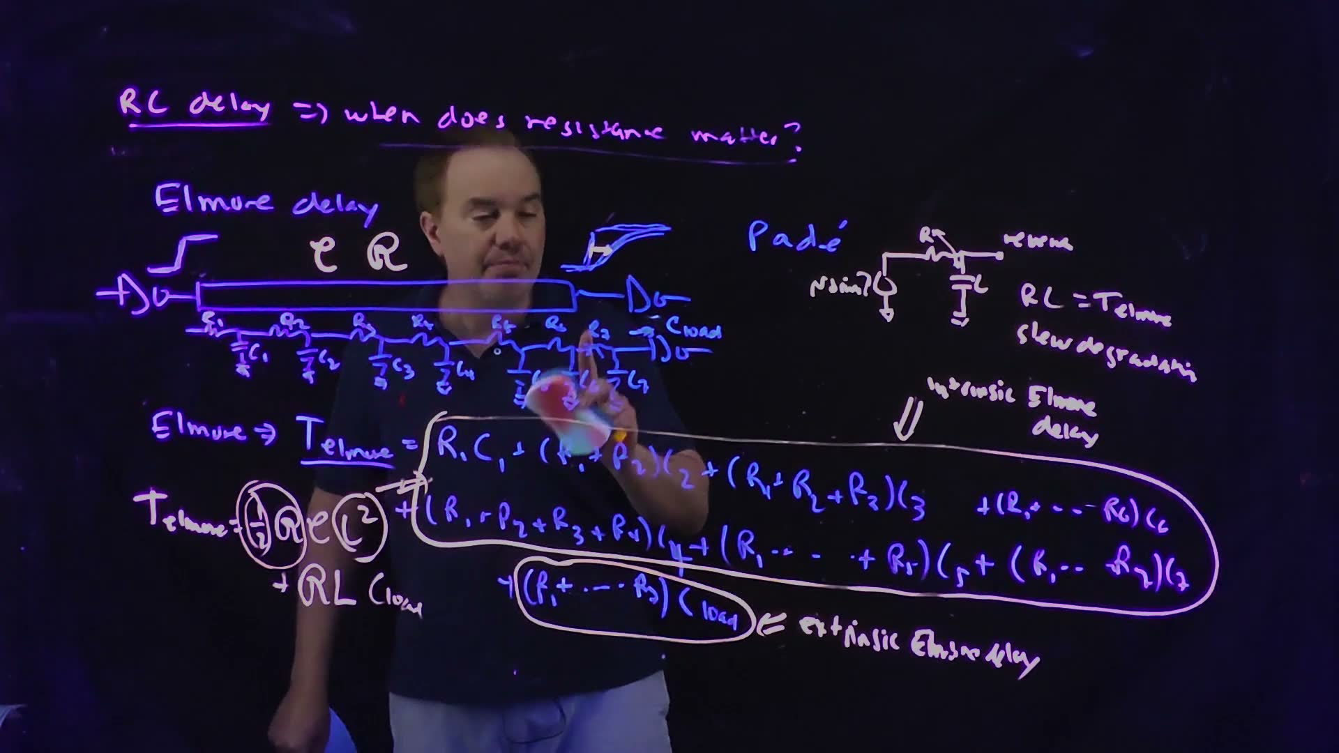
Fair copy of the board above (Lecture19 @ 27:59), mark for mark in its own layout. Black is the blue pen (the wire sketch, the ladder, “Padé” and the Elmore sum) and the violet pen (the title line). Magenta is the pale pink pen: what 24:23 and 24:39 drew in it (the arrow at the receiver’s edge, the loops and their labels, the single-pole circuit) and what was added by 27:59: $T_{elmore}$ after "$RC =$", “slew degradation”, the line’s $\mathcal{C}$ and $\mathcal{R}$ over the wire, and at the lower left the uniform-line formula $T_{elmore} = \frac{1}{2}\mathcal{R}\mathcal{C}L^2 + \mathcal{R}L\,C_{load}$RLCload​, with the ½ and the $L^2$ circled and two strokes towards the sum. The board also writes the ½ and the $L^2$ in parentheses inside their circles; the copy leaves the parentheses out, as at this size they merge with the circles. The lecturer’s hand covers $C_5$ to $C_7$ in the ladder and "$(R_1+R_2)$" in the sum’s first line; they are copied from 24:39. The writing is levelled; the board’s lines drift down to the right.

Where the ½ comes from added, computed from $r(x) = \mathcal{R}x$Rx. The resistance back to the driver rises linearly along the wire, so its average over the wire’s capacitance is half the total (dashed). A four-section ladder (dots) puts each capacitor at the end of its section, and averages $(k+1)/(2k) = 5/8$ (dotted).

Elmore delay of a uniform lineboard

$$T_{Elmore} = \underbrace{\tfrac12\,\mathcal{R}\mathcal{C}L^2}_{\text{intrinsic}} + \underbrace{\mathcal{R}L\,C_{load}}_{\text{extrinsic}} = \tfrac12 R\,C_w + R\,C_{load}$$

Holds when: one width and one environment along the whole wire (so ℛ and 𝒞 are constant), a lumped load at the far end; a wire with two widths is two segments (Sections 7 and 10)

Memorize or derive. Memorize the formula, and be ready to derive the ½ in three lines:

1. A slice $dx$ at $x$ has $\mathcal{C}\,dx$ and sees $\mathcal{R}x$Rx.
2. Add them up: $\int_0^L \mathcal{R}x\,\mathcal{C}\,dx = \tfrac12\mathcal{R}\mathcal{C}L^2$ (or the $k$-section sum above with $k \to \infty$∞).
3. Add the load, which sees all of $\mathcal{R}L$RL.

When does each part win? added The two parts are equal when $\tfrac12\mathcal{C}L = C_{load}$Cload​, that is when the wire’s own capacitance is twice the load. Shorter than that, the load term dominates; longer, the $L^2$ term does.

The $L^2$ growth added, computed for the lecture’s wire: $\mathcal{R} = 0.19\ \Omega/\mu$m, $\mathcal{C} = 0.1$ fF/µm, $C_{load} = 500$ fF. The intrinsic part, $9.5\ \text{ps}\cdot(L/\text{mm})^2$(L/mm)2, is small at 1 mm (9.5 ps against 95 ps, the dots) but catches the extrinsic part, $95\ \text{ps}\cdot(L/\text{mm})$(L/mm), at 10 mm, where the wire’s 1000 fF is twice the load.

A worked example added. The lecture’s wire from Section 5: $\mathcal{R} = 0.19\ \Omega/\mu$m, $\mathcal{C} = 0.1$ fF/µm, into $C_{load} = 500$ fF.

Doubling the length

1. At 1 mm. Intrinsic $\tfrac12 \times 0.19 \times 0.1 \times 1000^2\ \Omega\cdot\text{fF} = 9500\ \Omega\cdot\text{fF} = 9.5$ ps; extrinsic $190\ \Omega \times 500$ fF = 95 ps.
2. At 2 mm. Intrinsic $4 \times 9.5 = 38$ ps (the square); extrinsic $2 \times 95 = 190$ ps.
3. Where they meet. $C_w = 2C_{load}$ means $0.1L = 1000$ fF, $L = 10$ mm, where both parts are 950 ps.

Traps.

• Dropping the ½. $\mathcal{R}\mathcal{C}L^2$ is the one-section lump: all the resistance in front of all the capacitance. That is the $k = 1$ case, twice too big.
• Squaring $L$ in the extrinsic term. The load sits at one place and sees the resistance once: $\mathcal{R}L\,C_{load}$RLCload​.
• Mixed units. Keep Ω/µm, fF/µm and µm, multiply to Ω·fF, then divide by 1000 for ps.

Check yourself A uniform line has R = 500 Ω and C_w = 200 fF and no load. What is its Elmore delay?

$\tfrac12 \times 500 \times 200 = 50000\ \Omega\cdot\text{fF} = 50$ ps.

Check yourself For the lecture's wire (𝒞 = 0.1 fF/µm) driving 50 fF instead of 500 fF, at what length are the intrinsic and extrinsic parts equal?

When $C_w = 2C_{load} = 100$ fF: $L = 100/0.1 = 1000$ µm, 1 mm.

5. Worked example: a 1 mm point-to-point wire

You need

The uniform-line formula (Section 4). For a wire of one width with resistance $\mathcal{R}$ and capacitance $\mathcal{C}$ per unit length, length $L$L, driving a load $C_{load}$ at its far end:

$$T_{Elmore} = \tfrac12\mathcal{R}\mathcal{C}L^2 + \mathcal{R}L\,C_{load}.$$

The first term is the intrinsic part (the wire against itself), the second the extrinsic part (the wire against the load).

The uniform line (Lecture19 @ 27:59, redrawn): $\tfrac12\mathcal{R}\mathcal{C}L^2 + \mathcal{R}L\,C_{load}$RLCload​. Original figure ↑

Per-length resistance (Section 1). $\mathcal{R} = R_\square/W$R□​/W: the sheet resistance divided by the width.

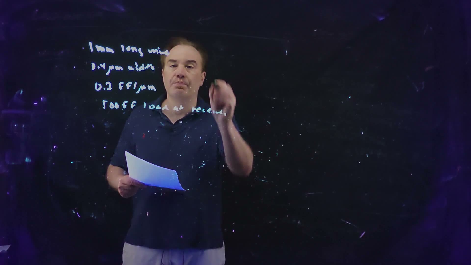
The question (the board’s givens, 40:11–41:20) board: a point-to-point wire, 1 mm long and 0.4 µm wide, with 0.1 fF/µm of capacitance and a sheet resistance of 0.076 Ω/□, drives a 500 fF load at its receiver. What is its Elmore delay?

The lecture’s point-to-point net added (values from the board, Lecture19 @ 45:26): 1 mm of 0.4 µm wire at 0.076 Ω/□ and 0.1 fF/µm into 500 fF. Below the wire, the per-length resistance and the totals the example computes.

The lecture's example (board, 41:30–43:58)

1. Which formula. “This is a point-to-point net”: one driver, one receiver, no branches, one width. The uniform-line formula applies, with the 500 fF as $C_{load}$Cload​.
2. Resistance per length. $\mathcal{R} = R_\square/W = 0.076/0.4 = 0.19\ \Omega/\mu$m, so the whole wire is $R = 0.19 \times 1000 = 190\ \Omega$190 Ω. (The board writes the fraction 0.076 Ω/□ over 0.4 µm in both terms; the speech says “times”, a slip.)
3. Intrinsic part. $\tfrac12 \times 0.19\ \Omega/\mu\text{m} \times 0.1\ \text{fF}/\mu\text{m} \times (1000\ \mu\text{m})^2 = 9500\ \Omega\cdot\text{fF} = 9.5$ ps board.
4. Extrinsic part. $190\ \Omega \times 500\ \text{fF} = 95000\ \Omega\cdot\text{fF} = 95$ ps board.
5. Total. $T_{Elmore} = 9.5 + 95 = 104.5$ ps board, “very significantly dominated by the extrinsic Elmore delay. It’s really resistance of the line acting against this rather substantial load” (43:58).

The board (Lecture19 @ 45:26)

Lecture19 @ 45:26The worked example: 9.5 ps intrinsic + 95 ps extrinsic = 104.5 ps. The givens' 0.1 fF/µm is written with a hooked 1 that looks like a 2; the working line's 0.1, the spoken 'a tenth of a femtofarad per micron' and the 9.5 ps all fix it as 0.1. The working line drops the /µm after 0.1 fF.

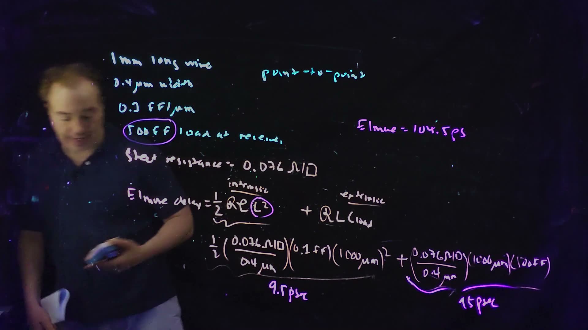
Fair copy of the board above (Lecture19 @ 45:26), mark for mark in its own layout. Black is the cyan pen: the givens and “point-to-point”. Magenta is two later pens that carry on one layer, the working: the pale pink pen (the sheet resistance, the Elmore formula with “intrinsic” and “extrinsic”, the intrinsic half of the numbers) and the violet pen (the extrinsic half, the circles round 500 fF and $L^2$L2, “9.5 psec”, “95 psec” and “Elmore = 104.5 ps”). Two slips are marked †. The givens’ 0.2† is 0.1 fF/µm, written with a hooked 1 that reads like a 2: the working line’s 0.1, the spoken “a tenth of a femtofarad per micron” and the 9.5 ps all need 0.1. The working line’s (0.1 fF†) drops the unit’s /µm; it is 0.1 fF/µm. The sheet-resistance line and the working line are levelled.

Check added. Two independent routes.

• A bound. Lump all the capacitance at the far end, so that everything sees the whole 190 Ω: $190 \times (100 + 500)$ fF = 114 ps. The real wire’s own capacitance sees only half of it on average, so the Elmore delay must be below 114 ps: 104.5 is.
• Which part should win. Section 4’s rule: the intrinsic part wins only when the wire’s capacitance exceeds twice the load. Here $C_w = 100$ fF against $2 \times 500 = 1000$ fF, so the extrinsic part must dominate, and it does, 95 against 9.5 ps.

About the numbers. The lecturer adds that 0.076 Ω/□ “is actually a little high. This would be more like aluminum interconnect than copper” (41:06). Copper’s lower levels are nearer the 0.04 Ω/□ of Section 1.

Traps.

• Reading the handwritten givens’ “0.1” as 0.2 fF/µm. That would give 19 ps intrinsic, not the board’s 9.5 ps.
• Attacking the intrinsic part first. It is 9% of the total. The lever here is the resistance against the 500 fF load: a lower $\mathcal{R}$ (a wider wire, Section 8, or a lower-resistance layer).

Check yourself The same wire drives 250 fF instead of 500 fF. What is its Elmore delay?

The intrinsic part is unchanged, 9.5 ps; the extrinsic part halves, $190 \times 250$ fF = 47.5 ps. $T_{Elmore} = 57$ ps.

Check yourself The same 1 mm, 0.4 µm wire is moved to a copper layer of 0.04 Ω/□. What are its ℛ and its Elmore delay into 500 fF?

$\mathcal{R} = 0.04/0.4 = 0.1\ \Omega/\mu$m, $R = 100\ \Omega$100 Ω. Intrinsic $\tfrac12 \times 100 \times 100$ fF = 5 ps; extrinsic $100 \times 500$ fF = 50 ps; $T_{Elmore} = 55$ ps.

6. When resistance matters: Elmore delay against the slew

You need

The single-pole receiver model (Section 3). The receiver’s waveform is the driver’s waveform passed through one RC with $RC = T_{Elmore}$TElmore​. The delay is about $T_{Elmore}$TElmore​, and the edge gets slower by about $2T_{Elmore}$ (a step through one pole $\tau$ takes $2.2\tau$ from 10% to 90%).

The receiver’s model (Lecture19 @ 24:39, redrawn): the driver’s waveform through one RC equal to $T_{Elmore}$TElmore​. Original figure ↑

The lecture’s example (Section 5). 1 mm of 0.4 µm wire at 0.076 Ω/□ and 0.1 fF/µm into 500 fF: $T_{Elmore} = 9.5 + 95 = 104.5$ ps.

The FO1 delay (Chapter 7). $\tau_{inv}$τinv​, the delay of an inverter driving one copy of itself, is the technology’s unit of gate delay. A gate’s output edge takes a few gate delays to switch.

The question. Extracting resistance is expensive, and ignoring it can be wrong. Is there a quick test for whether a wire’s resistance matters?

Compare the Elmore delay with the slew (board, 28:00–33:30)

1. The test. The board boxes the question, “when does resistance matter?”, and answers it with “slew rate ⇔ Elmore delay” board. The lecturer’s “slew rate” is a time: how long the edge takes to switch, in picoseconds (this chapter writes $t_r$tr​). “If my Elmore delay is much less than my slew rate, then I don’t need to worry about any of this … The resistance of the line just doesn’t matter” (29:25). If the Elmore delay is comparable to the slew or larger, it matters.
2. What the test means. Feed the lecture’s 104.5 ps pole two different edges added. A 300 ps ramp comes out about 94 ps late, close to $T_{Elmore}$ itself, and its 10–90% time is stretched by about 40%, from 240 to 334 ps: a real effect, but small next to the edge, which is still mostly the driver’s. A 50 ps ramp comes out with a 10–90% time of 233 ps, almost six times its own 40 ps: the wire, not the driver, now decides the edge. That is the lecturer’s answer to his own question: for a 200–300 ps slew, “would I care about the resistance of this line? No”; for 50 ps, “the answer is unequivocally yes” (44:19–44:35).
3. Resistive shielding. Resistance does a second thing (28:52–30:52). When the edge is fast, the far end of the wire is “so electrically far away” that the driver finishes its edge before that capacitance has charged. The driver does not see the whole $C_1 + \dots + C_7 + C_{load}$Cload​: part of it is shielded by the resistance in between board.
4. The π model. So instead of one capacitor, the driver sees a π model: $C_{near}$ at its output, a series resistance $R$R, then $C_{far}$Cfar​, with $C_{near} + C_{far}$ equal to the total (31:27–32:13) board. Static-timing tools use it to size drivers. The course does not derive its values: “I used to go through how you would derive this … but I don’t do that anymore. I think it’s a little bit too … into the weeds” (32:17).
5. The test in exam form added. A paper rarely gives the slew. It gives the technology’s gate delay, often the FO1 delay. Edges last a few gate delays, so: a $T_{Elmore}$ well below one FO1 delay means the resistance can be ignored, and the wire is a lumped capacitance; a $T_{Elmore}$ of several FO1 delays means it must be included.

The receiver’s waveform for slow and fast edges added, computed from a linear ramp of rise time $t_r$ through one pole $\tau = T_{Elmore} = 104.5$ ps (the lecture’s example). (a) $t_r = 300$ ps: the output is 94.4 ps later, about $T_{Elmore}$TElmore​, and its edge is stretched by about 40% (10–90% in 333.7 ps against 240 ps), small next to the edge. (b) $t_r = 50$ ps: the output’s edge is set by the wire (10–90% in 232.5 ps against 40 ps), and the delay is 73.4 ps.

The π model of a resistive wire, as its driver (the inverter at the left) sees it, redrawn from the board (Lecture19 @ 33:54). $C_{near} + C_{far}$ is the total capacitance; $R$ shields $C_{far}$ from a fast driver.

The board (Lecture19 @ 33:54)

Lecture19 @ 33:54The finished Elmore board: the question boxed, 'slew rate ⇔ Elmore delay', resistive shielding and the π model (C_near, R, C_far) in cyan.

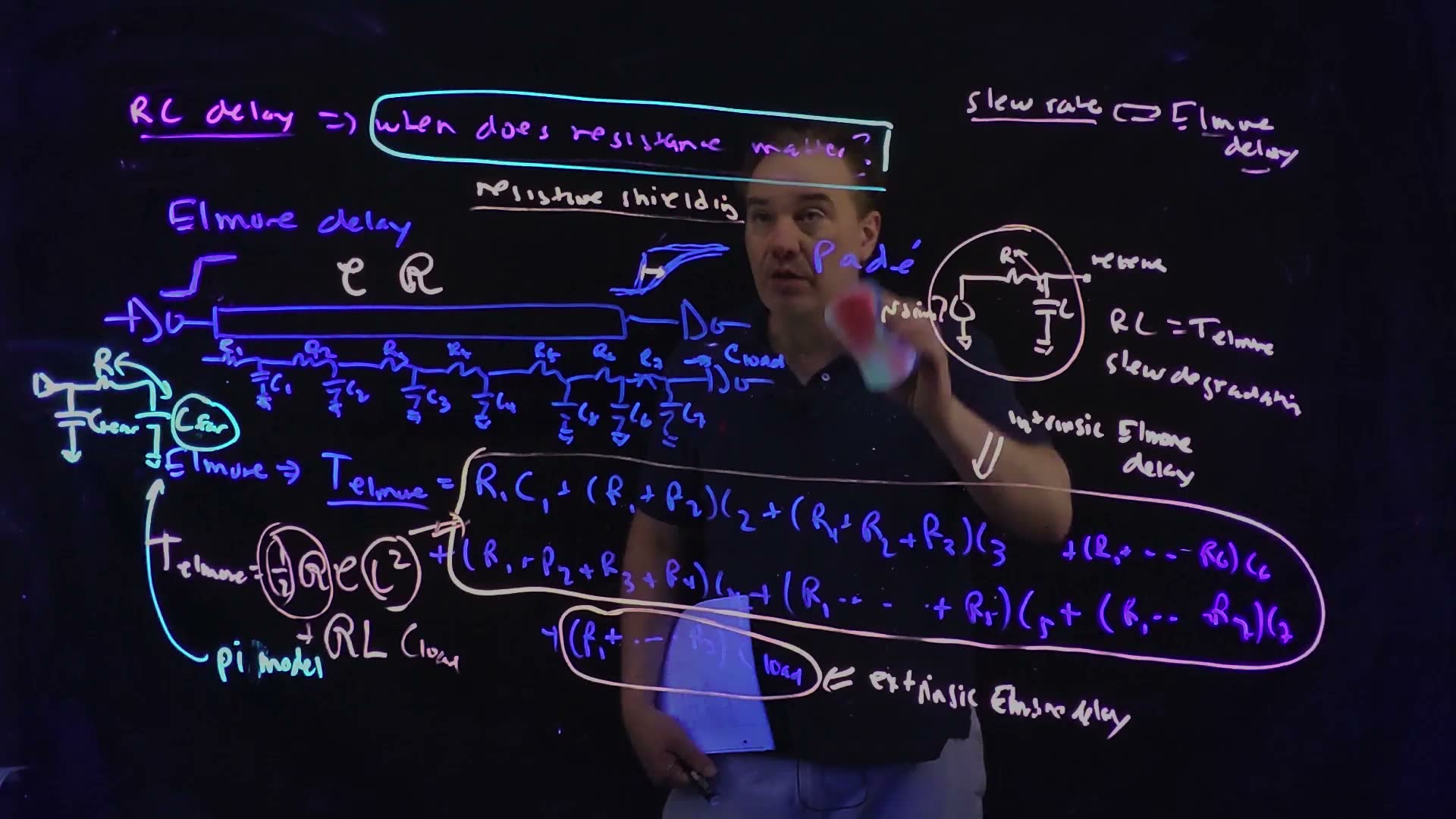
Fair copy of the board above (Lecture19 @ 33:54), mark for mark in its own layout. Black is the blue pen (the wire sketch, the ladder, “Padé” and the Elmore sum) and the violet pen (the title line). Magenta is the pale pink pen: the marks of 24:23 to 27:59 (the loops and their labels, the single-pole circuit with "$RC = T_{elmore}$" and “slew degradation”, $\mathcal{C}$ and $\mathcal{R}$R, the uniform-line formula) and, new by 33:54, “resistive shielding”, “slew rate ⇔ Elmore delay” and the circle round the single-pole circuit. Teal is the cyan pen, a separate layer: the box round “when does resistance matter?” and, at the left, the π model (a driver, $C_{near}$Cnear​, $R$ with an arrow to the circled $C_{far}$Cfar​) with “pi model” and its arrow. The lecturer’s hand hides “driver?” and the sheet he holds hides the middle of the $C_{load}$ term in this frame; both are copied from 27:59. The circle round the single-pole circuit is broken where it crosses “driver?”, and, as at 27:59, the parentheses round the ½ and the $L^2$ inside their circles are left out. The writing is levelled; the board’s lines drift down to the right.

When resistance mattersboard

$$\begin{aligned} T_{Elmore} \ll t_r &: \ \text{a lumped capacitance} \\ T_{Elmore} \gtrsim t_r &: \ \text{include } R \text{ (delay, slew, shielding)} \end{aligned}$$

Holds when: an order-of-magnitude test, not a sharp threshold; t_r is the edge's transition time (the lecturer's slew rate)

Memorize or derive. Memorize the test, and that the π model is $C_{near}$Cnear​, $R$R, $C_{far}$ with $C_{near} + C_{far}$ the total.

A worked example added, both ends of the test.

A long wire and a short one

1. The lecture’s 1 mm wire, $T_{Elmore} = 104.5$ ps. Against a 300 ps edge the wire adds 94.4 ps of delay but leaves the edge’s shape mostly alone; against a 50 ps edge it stretches the edge to 232.5 ps (10–90%). With 50 ps edges the resistance must be in the model.
2. A 100 µm piece of the same wire into 20 fF. $R = 0.19 \times 100 = 19\ \Omega$19 Ω, $C_w = 0.1 \times 100 = 10$ fF. Intrinsic $\tfrac12 \times 19 \times 10 = 95\ \Omega\cdot\text{fF} = 0.095$ ps; extrinsic $19 \times 20 = 380\ \Omega\cdot\text{fF} = 0.38$ ps; $T_{Elmore} = 0.475$ ps. Against any real edge this is nothing: treat the piece as 10 fF of extra load, 30 fF in all, and forget its resistance.

Check. Scaling from Section 5 gives step 2 independently: a tenth of the length makes the intrinsic part a hundredth (9.5 → 0.095 ps), and the extrinsic part is $19\ \Omega$ against 20 fF instead of 190 Ω against 500 fF, $1/250$ of 95 ps = 0.38 ps.

Traps.

• Reading “slew rate” as volts per picosecond. Then the test comes out backwards. Here it is a time, and a short slew (a fast edge) is the case where resistance matters.
• “The resistance doesn’t matter” read as “the wire doesn’t matter”. Its capacitance still loads the driver, always.
• Trying to compute $C_{near}$ and $C_{far}$Cfar​. The course does not, and no paper asks.

Check yourself A net's Elmore delay is 5 ps and its edges take 100 ps. Does its resistance matter?

No: 5 ps is far below the 100 ps slew. Model the wire as a lumped capacitance.

Check yourself A technology's FO1 delay is 20 ps. A long wire's Elmore delay is 150 ps. About how many FO1 delays is that, and must the wire's resistance be included?

$150/20 = 7.5$ FO1 delays. Edges last a few gate delays, so the wire’s delay is comparable to or longer than any edge: yes, include the resistance.

7. Trees and side branches

You need

The Elmore rule (Section 3). Each capacitance counts with the resistance between it and the driver; the receiver’s load with the whole resistance.

The ladder (Lecture19 @ 24:23, redrawn): each $C_i$ counts with $R_1 + \dots + R_i$Ri​. Original figure ↑

The uniform line (Section 4). A uniform segment with total resistance $R$ and capacitance $C_w$ contributes $\tfrac12RC_w$ against itself: its capacitance sees, on average, half its resistance.

The uniform line (Lecture19 @ 27:59, redrawn): a slice at $x$ sees $\mathcal{R}x$Rx. Original figure ↑

A gate driving a load (Chapter 7). An inverter of input capacitance $C_{in}$ drives a load $C_{load}$ in $\tau_{inv}\,C_{load}/C_{in}$τinv​Cload​/Cin​, with $\tau_{inv}$ the FO1 delay. With no resistive shielding (Section 6), the gate that drives a whole tree sees the tree’s total capacitance as its load.

The question. Most nets have one driver and several receivers (a multi-drop net). How does the Elmore delay handle the branches?

A net with two receivers (board, 34:55–39:19)

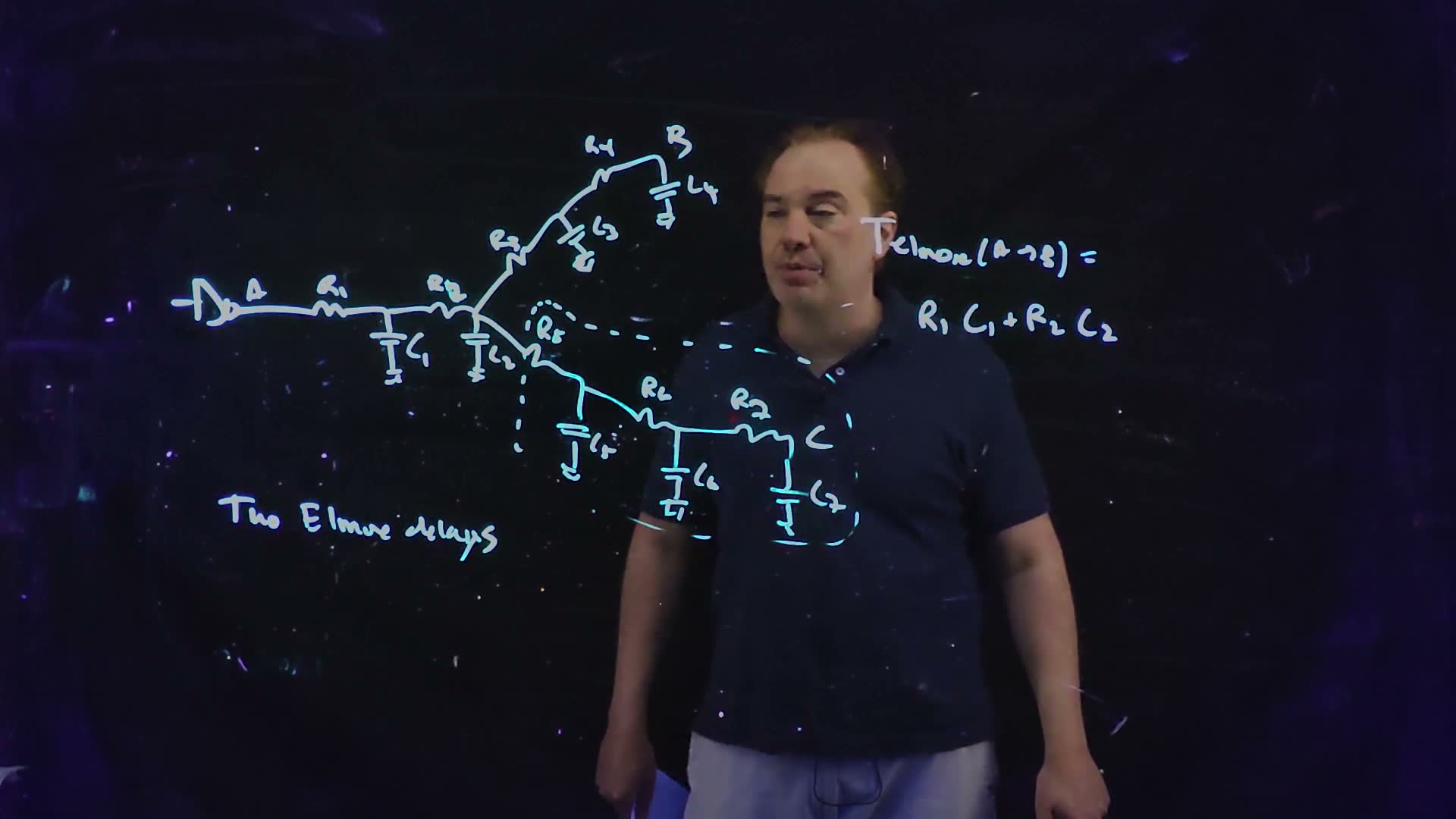
1. The net. A driver at A, a trunk ($R_1$R1​, $C_1$C1​, $R_2$R2​, then $C_2$ at the branch node), and two branches: up through $R_3$R3​, $C_3$C3​, $R_4$ to B with $C_4$C4​; down through $R_5$R5​, $C_5$C5​, $R_6$R6​, $C_6$C6​, $R_7$ to C with $C_7$ board. The receivers’ input capacitance is folded into $C_4$ and $C_7$C7​. “There are two Elmore delays in play here”: A→B and A→C (36:26).
2. A→B: lump the side branch. For B, the trunk and the up branch are the path; the down branch is a side branch. “I’m going to take all of this capacitance and … pull it up to this node” (37:16): the whole side branch’s capacitance counts with the resistance up to the branch node, $R_1 + R_2$R2​. The board’s sum (39:26), after a false start at 37:59: $\begin{aligned}T_{Elmore}(A{\to}B) = {} & R_1C_1 + (R_1{+}R_2)(C_2{+}C_5{+}C_6{+}C_7) \\ & + (R_1{+}R_2{+}R_3)C_3 + (R_1{+}R_2{+}R_3{+}R_4)C_4.\end{aligned}$ Why the side branch’s own resistors $R_5$R5​, $R_6$R6​, $R_7$ do not appear: the current into $C_5$C5​, $C_6$C6​, $C_7$ does flow through them, but on the way to B only the shared $R_1 + R_2$ is crossed. The side branch’s resistance also shields its capacitance a little, but a single pole “cannot capture that effect”; a two-pole model can, and some CAD tools use one (37:16–37:43).
3. A→C, the other way round. Spoken, not written (38:52): now the up branch is the side branch. $\begin{aligned}T_{Elmore}(A{\to}C) = {} & R_1C_1 + (R_1{+}R_2)(C_2{+}C_3{+}C_4) + (R_1{+}R_2{+}R_5)C_5 \\ & + (R_1{+}R_2{+}R_5{+}R_6)C_6 + (R_1{+}R_2{+}R_5{+}R_6{+}R_7)C_7.\end{aligned}$ Both sums follow one rule: every capacitance counts with the resistance it shares with the path from the driver to the receiver.
4. Distributed trees: the segment form added. Exam trees are drawn as uniform segments with lengths, not as lumps. Regroup the same sum by path segment: segment $k$ of the path, with resistance $R_k$ and capacitance $C_k$Ck​, carries the charging current of everything beyond its far end, $C_{down,k}$ (side branches that leave further along included), and of its own capacitance at half weight. So $T_{Elmore}(A{\to}B) = \sum_{k\,\in\,\text{path}} R_k\Big(\tfrac12 C_k + C_{down,k}\Big).$ Off-path resistances never appear. A lumped capacitor halfway along a segment splits that segment into two.

A net with two receivers, redrawn from the board (Lecture19 @ 39:26). For the delay to B, the down branch is a side branch: its whole capacitance, $C_5 + C_6 + C_7$C7​, is lumped at the branch node (the dashed box and arrow) and counts with $R_1 + R_2$R2​. The receivers’ input capacitance is part of $C_4$ and $C_7$C7​.

The board (Lecture19 @ 39:26)

Lecture19 @ 39:26The multi-drop net: two Elmore delays, and the A→B sum with the side branch lumped at the branch node.

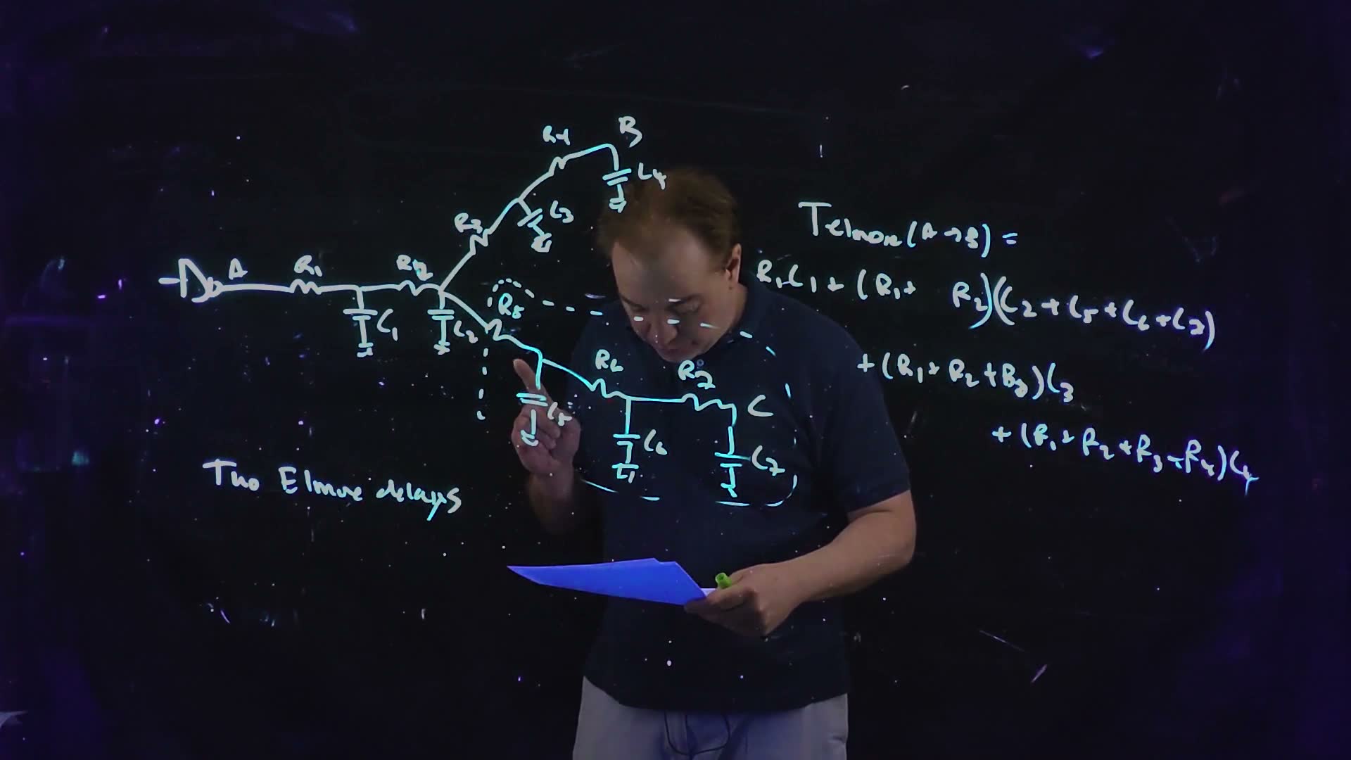
Fair copy of the board above (Lecture19 @ 39:26), mark for mark in its own layout. One pen (cyan), copied in black. The dashed loop marks the side branch to C, whose capacitance $C_5+C_6+C_7$ is lumped at the branch node in the sum for $A\to B$B. The head hides the middle of the loop’s upper edge and the hand the label $C_5$ in this frame; they are copied from 38:44. On the board the first line of the sum has a gap before $R_2$R2​, which is left over from the first start, $R_1C_1+R_2C_2$ (37:59); the copy closes it up. The sum’s lines are levelled.

The segment form added. Segment 2’s resistance $R_2$ carries the charging current of its own capacitance (at half weight) and of everything beyond its far end, $C_{down,2}$Cdown,2​: segment 3 and $C_{load}$Cload​. The side branch leaves before segment 2, so it is in $C_{down,1}$ but not in $C_{down,2}$Cdown,2​.

Elmore delay to one receiver of a treeboard

$$T_{Elmore}(A{\to}B) = \sum_{\text{every } c} c \times R_{shared}(c,\,B)$$

where $R_{shared}(c, B)$ is the resistance that $c$‘s path to the driver shares with the path from A to B.

Holds when: all capacitances grounded; a single pole (the side branch's own shielding is not captured)

The segment formadded

$$T_{Elmore}(A{\to}B) = \sum_{k\,\in\,\text{path}} R_k\left(\tfrac12 C_k + C_{down,k}\right)$$

Holds when: a tree of uniform segments; each path segment k has resistance R_k and capacitance C_k; C_down,k is everything beyond its far end, side branches included

Memorize or derive. Memorize the shared-resistance rule. Derive the segment form when you need it:

1. Each capacitance counts with the path resistance it shares with B’s path.
2. Collect the terms by path resistor: $R_k$ multiplies every capacitance whose charging current crosses it, which is everything beyond segment $k$k.
3. A segment’s own capacitance sees, on average, half of $R_k$ (Section 4).

A worked example added. A tree of 0.4 µm wire at 0.076 Ω/□ (0.19 Ω/µm) and 0.1 fF/µm: A to X is 500 µm; from X, a branch of 1000 µm to B with 50 fF, and a branch of 1500 µm to C with 20 fF.

The worked example’s tree added. For the delay to B the path is A–X–B (thick); the branch to C (dashed) is a side branch, lumped at X with its wire and its 20 fF. Each branch’s length (1000 µm, 1500 µm) includes its short riser; the arrows span only the horizontal runs.

Two Elmore delays in a tree

1. The segments. A–X: $R = 0.19 \times 500 = 95\ \Omega$95 Ω, $C = 0.1 \times 500 = 50$ fF. X–B: 190 Ω, 100 fF. X–C: 285 Ω, 150 fF.
2. A→B, segment A–X. Everything beyond X: X–B’s 100 fF, B’s 50 fF, X–C’s 150 fF and C’s 20 fF, 320 fF in all. $95 \times (\tfrac12 \cdot 50 + 320) = 95 \times 345 = 32775\ \Omega\cdot\text{fF} = 32.775$ ps (2.375 ps of it against its own capacitance, 30.4 ps against the rest).
3. A→B, segment X–B. Beyond it only B’s 50 fF: $190 \times (50 + 50) = 19$ ps (9.5 against itself, 9.5 against the load).
4. $T_{Elmore}(A{\to}B) = 32.775 + 19 = 51.775$ ps. The branch to C is not on B’s path, but its wire and load, $150 + 20 = 170$ fF, still cost $95 \times 170\ \Omega\cdot\text{fF} = 16.15$ ps through the trunk. (The trunk’s 30.4 ps against everything beyond X also includes B’s own branch.)
5. A→C. The A–X term is the same, 32.775 ps, because its downstream capacitance is the same. X–C: $285 \times (\tfrac12 \cdot 150 + 20) = 285 \times 95 = 27.075$ ps. $T_{Elmore}(A{\to}C) = 59.85$ ps.

Check. Recompute A→B by the shared-resistance rule, capacitance by capacitance: A–X’s own 50 fF at half of 95 Ω, 2.375 ps; the 170 fF of the C branch and its load at 95 Ω, 16.15 ps; X–B’s 100 fF at $95 + 95$ Ω on average, 19 ps; B’s 50 fF at $95 + 190$ Ω, 14.25 ps. The sum is 51.775 ps, as before. And C, at the end of the longer branch, is the later receiver.

Traps.

• Putting the side branch’s resistance into the delay ($R_5$R5​, or X–C’s 285 Ω, in A→B). Only the shared resistance counts.
• Leaving the side branch out altogether. Its capacitance still loads the shared trunk: 16.15 ps of the 51.775 ps above.
• One ½RC for a whole path of mixed widths. When the segments differ (one is widened), use the segment form, segment by segment.

Check yourself In the board's net, which resistances multiply C₆ in the Elmore delay from A to B?

$R_1 + R_2$R2​: the resistance $C_6$‘s path to the driver shares with the path to B. $R_5$ and $R_6$ are on the side branch.

Check yourself In the worked example, add 30 fF halfway along the X–B branch (500 µm from X). What are the new delays to B and to C?

For B, the 30 fF sees the trunk and half the branch, $95 + 95 = 190\ \Omega$190 Ω: $+5.7$ ps, so $T_{Elmore}(A{\to}B) = 57.475$ ps. For C it is on a side branch and sees only the trunk’s 95 Ω: $+2.85$ ps, so $T_{Elmore}(A{\to}C) = 62.7$ ps.

Check yourself Why can't the Elmore delay capture the shielding of a side branch by its own resistance?

It is a single-pole estimate: one number, one pole. Describing how the side branch’s resistance hides part of its capacitance would need a second pole (the lecturer: “a two-pole approximate”).

8. Fix 1: widening the wire

You need

The uniform line (Section 4). $T_{Elmore} = \tfrac12\mathcal{R}\mathcal{C}L^2 + \mathcal{R}L\,C_{load}$RLCload​: the intrinsic part (the wire against itself) and the extrinsic part (the wire against the load).

The uniform line (Lecture19 @ 27:59, redrawn). Original figure ↑

Per-length resistance (Section 1). $\mathcal{R} = R_\square/W$R□​/W: twice the width, half the resistance.

Parallel-plate capacitance added. Proportional to the facing area over the gap.

The lecture’s example (Section 5). 1 mm of 0.4 µm wire at 0.076 Ω/□ into 500 fF: 9.5 + 95 = 104.5 ps.

The question. “My Elmore delay is really bad. What do I do?” (45:52). The first answer is to widen the wire. What does that buy, and what does it cost?

What widening does (board, 46:11–50:22)

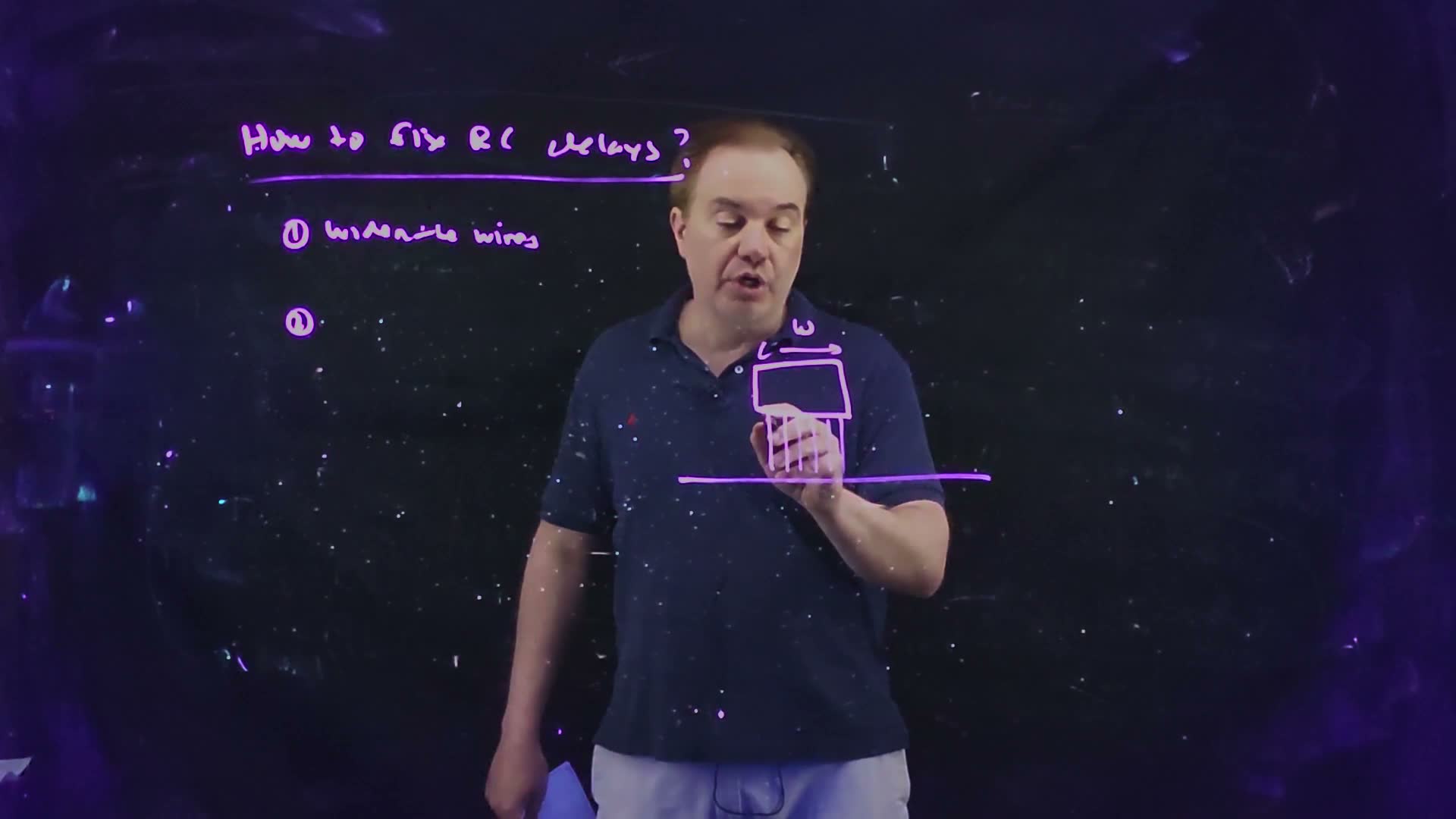
1. The extrinsic part always falls. A wider wire has proportionally less resistance, and the load does not change, so $\mathcal{R}L\,C_{load}$ falls as $1/W$1/W: “a definite win” (46:51) board.
2. The capacitance has two parts. Look at the wire’s cross-section above the substrate (or a neighbour). Field lines run straight down from its bottom face: the areal part, proportional to the width. Field lines also curve out from its sides: the fringe part, which “doesn’t care at all about the width” (47:32–48:51). So board $C = C_{areal}\cdot W\cdot L + C_{fringe}\cdot L,$ with $C_{areal}$ per unit area and $C_{fringe}$ per unit length. This is the form a paper writes as, for example, "$0.04\ \text{fF}/\mu\text{m} + 0.15\ \text{fF}/\mu\text{m}^2 \times W$".
3. The intrinsic part falls only in its fringe share. Put $\mathcal{R} = R_\square/W$ and $\mathcal{C} = C_{areal}W + C_{fringe}$ into $\tfrac12\mathcal{R}\mathcal{C}L^2$21​RCL2: $\tfrac12\,\frac{R_\square}{W}\,(C_{areal}W + C_{fringe})\,L^2 = \tfrac12 R_\square\Big(C_{areal} + \frac{C_{fringe}}{W}\Big)L^2.$ The areal part does not depend on $W$ (the resistance falls as fast as the areal capacitance grows); only the fringe part falls (49:08) board. However wide the wire, the intrinsic part never drops below $\tfrac12 R_\square C_{areal}L^2$21​R□​Careal​L2.
4. A number for it added. Give the lecture’s wire a fringe capacitance of 0.05 fF/µm and an areal capacitance of 0.125 fF/µm², so that at 0.4 µm it has the lecture’s 0.1 fF/µm. Its total delay falls from 104.5 ps at 0.4 µm to 24.7 ps at 2 µm and 14.7 ps at 4 µm; the intrinsic part creeps down towards its floor of 4.75 ps, the extrinsic part falls as $1/W$1/W.
5. The costs. A wider wire takes more routing tracks, and its total capacitance grows, so “I’m going to have to have a bigger driver, I’m going to burn more power” (50:03). “The only way to fix RC delay is unfortunately to consume power” (50:24).

The two parts of a wire’s capacitance, redrawn from the board (Lecture19 @ 49:19). Field lines from the bottom face give the areal part, $C_{areal}WL$Careal​WL, which grows with the width (↑); the fringing lines from the sides give $C_{fringe}L$Cfringe​L, which the board marks “constant”: it does not depend on $W$W.

The board (Lecture19 @ 49:19)

Lecture19 @ 49:19Widening: the areal capacitance grows with W, the fringe capacitance does not.

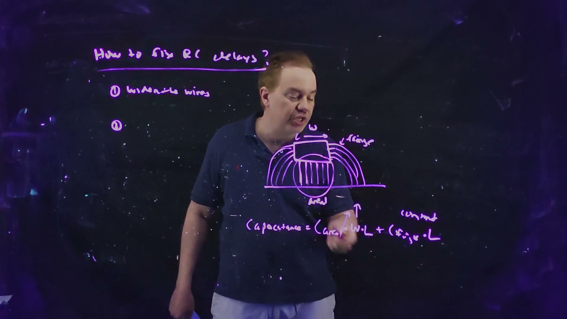
Fair copy of the board above (Lecture19 @ 49:19), mark for mark in its own layout. One pen (violet), copied in black. The circle groups the straight field lines under the wire, the areal part, which grows with the width $W$ (the two up arrows); the arcs from the side faces are the fringe part, which stays constant. The lecturer’s hand covers “areal ·” and the foot of the slanted arrow in the capacitance line in this frame; they are copied from 51:03. The ② is still empty: “repeater insertion” follows at 51:03. The capacitance line is levelled.

Widening the lecture’s wire added, computed from $T(W) = \tfrac12R_\square(C_{areal} + C_{fringe}/W)L^2 + (R_\square/W)LC_{load}$ with $R_\square = 0.076$ Ω/□, $C_{fringe} = 0.05$ fF/µm, $C_{areal} = 0.125$ fF/µm² (0.1 fF/µm at 0.4 µm), $L = 1$ mm, $C_{load} = 500$ fF. The extrinsic part falls as $1/W$1/W; the intrinsic part only towards its floor $\tfrac12 R_\square C_{areal}L^2 = 4.75$ ps (dashed).

Wire capacitance with widthboard

$$C = C_{areal}\,W L + C_{fringe}\,L$$

Holds when: capacitance to a plane (or a neighbour) below the wire; C_areal per unit area of the bottom face, C_fringe per unit length of the sides

Elmore delay against widthadded

$$T(W) = \tfrac12 R_\square\left(C_{areal} + \frac{C_{fringe}}{W}\right)L^2 + \frac{R_\square}{W}\,L\,C_{load}$$

Holds when: a uniform wire of width W and length L into C_load; ℛ = R_□/W and 𝒞 = C_areal·W + C_fringe

Memorize or derive. Memorize the capacitance form and what each term is. Derive $T(W)$ in two lines: substitute $\mathcal{R} = R_\square/W$ and $\mathcal{C} = C_{areal}W + C_{fringe}$ into the uniform-line formula, and cancel the $W$ in the areal term.

A worked example added, with the plot’s constants: widen the lecture’s 1 mm wire from 0.4 µm to 2 µm.

Widening from 0.4 µm to 2 µm

1. The new per-length values. $\mathcal{R} = 0.076/2 = 0.038\ \Omega/\mu$m; $\mathcal{C} = 0.125 \times 2 + 0.05 = 0.3$ fF/µm.
2. Intrinsic. $\tfrac12 \times 0.038 \times 0.3 \times 1000^2 = 5700\ \Omega\cdot\text{fF} = 5.7$ ps (from 9.5 ps).
3. Extrinsic. $0.038 \times 1000 = 38\ \Omega$38 Ω; $38 \times 500$ fF = 19 ps (from 95 ps).
4. Total. 24.7 ps, against 104.5 ps at 0.4 µm.
5. The cost. The wire’s own capacitance grows from 100 fF to $0.3 \times 1000 = 300$ fF: three times the charge to move on every edge, and a driver that must be stronger to keep its own delay.

Check. The extrinsic part scales as $1/W$1/W: $95 \times 0.4/2 = 19$ ps ✓. The intrinsic part must lie between its floor, 4.75 ps, and its old 9.5 ps: 5.7 ps ✓.

Traps.

• Expecting the intrinsic part to fall as $1/W$1/W. Only its fringe share does; the areal share stays.
• Forgetting the driver. The wire’s Elmore delay falls, but the driver now charges more capacitance, so its own delay grows (unless it is made bigger, which costs power).
• Keeping 0.1 fF/µm after widening. When a paper gives $C$ as a function of $W$W, recompute $\mathcal{C}$ at the new width.

Check yourself Suppose a wire's capacitance were all fringe (C_areal = 0). What would doubling its width do to its intrinsic Elmore delay?

Halve it: $\tfrac12 R_\square (C_{fringe}/W) L^2$ falls as $1/W$1/W. With no areal part there is no floor.

Check yourself For the lecture's wire with the constants above, at what width does the extrinsic part fall to 10 ps, and what is the total delay there?

The extrinsic part is $(0.076/W) \times 1000 \times 500$ fF = $38/W$ ps, so $W = 3.8$ µm. The intrinsic part is $38 \times (0.125 + 0.05/3.8) = 5.25$ ps, so the total is 15.25 ps.

9. Fix 2: repeaters

You need

The $L^2$ growth (Section 4). A uniform line’s intrinsic Elmore delay is $\tfrac12\mathcal{R}\mathcal{C}L^2$21​RCL2: double the length, four times the delay. For the lecture’s wire ($\mathcal{R} = 0.19\ \Omega/\mu$R=m, $\mathcal{C} = 0.1$ fF/µm) it is $9.5\ \text{ps}\cdot(L/\text{mm})^2$(L/mm)2.

The $L^2$ growth for the lecture’s wire (computed): $9.5\ \text{ps}\cdot(L/\text{mm})^2$ intrinsic. Original figure ↑

The question. Widening attacks $\mathcal{R}$R. The other lever is the $L^2$ itself: can a long wire be made to behave like several short ones?

Breaking the wire (board, 50:42–51:46)

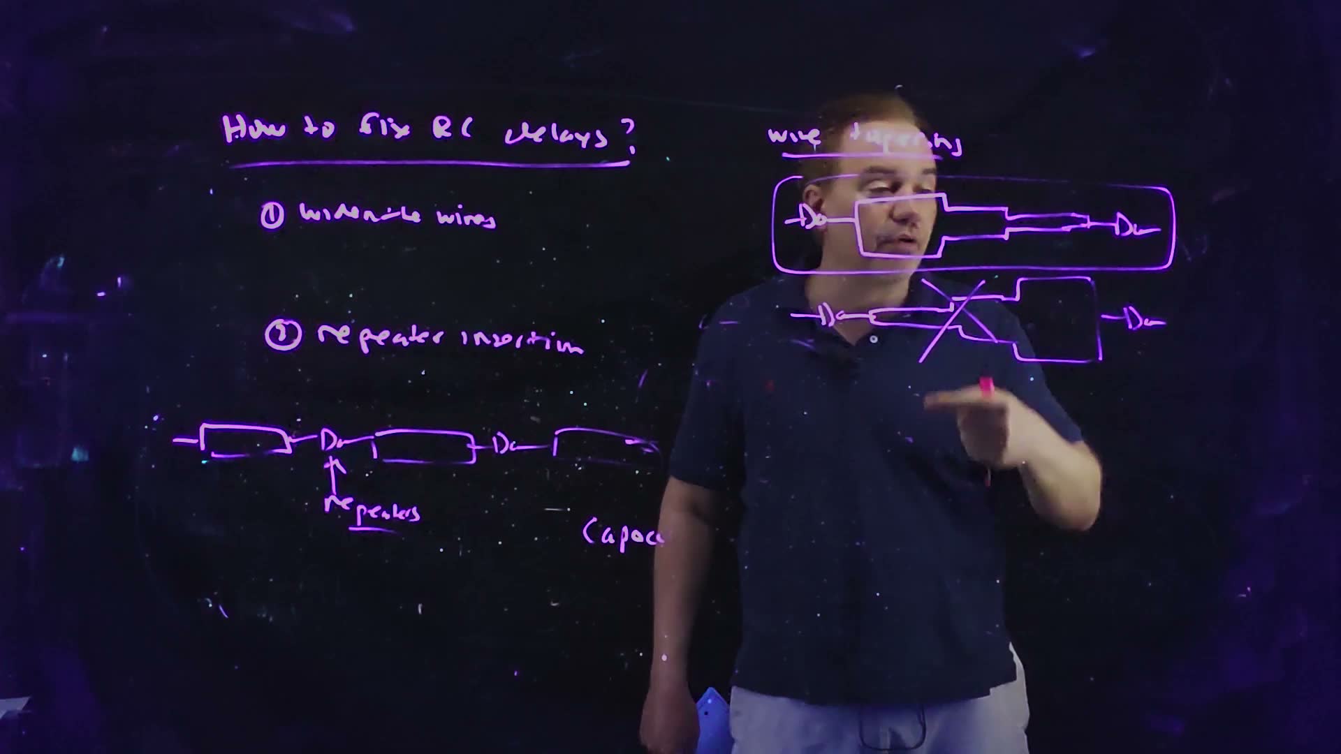
1. Repeaters. “Take the wire and break it up into segments and insert inverters” (50:42): the inverters are called repeaters board. Each one drives only its own piece of wire.
2. The wire part, $L^2$ into $L$ added. Cut a wire into $k$ equal pieces. Each piece’s intrinsic delay is $\tfrac12\mathcal{R}\mathcal{C}(L/k)^2$21​RC(L/k)2, and there are $k$ of them: $k \cdot \tfrac12\mathcal{R}\mathcal{C}(L/k)^2 = \tfrac1k\cdot\tfrac12\mathcal{R}\mathcal{C}L^2$21​RCL2. The wire’s own delay now grows linearly with its length (for a fixed piece length), not as its square.
3. The price. Each repeater adds its own gate delay, and each piece now drives the next repeater’s input capacitance. “Under the right conditions … adding these repeaters will actually reduce the overall delay” (51:19). How many repeaters, and how big, is the next lecture’s derivation (Chapter 21). They also cost power, a “not insignificant” share of a microprocessor’s (12:52).

Repeater insertion, redrawn from the board (Lecture19 @ 52:02). The long wire is cut into pieces with an inverter (a repeater, arrowed) after each, so each piece’s $L^2$ is a short one.

The board (Lecture19 @ 52:02)

Lecture19 @ 52:02The two fixes: widening (the cross-section) and repeater insertion (the chain).

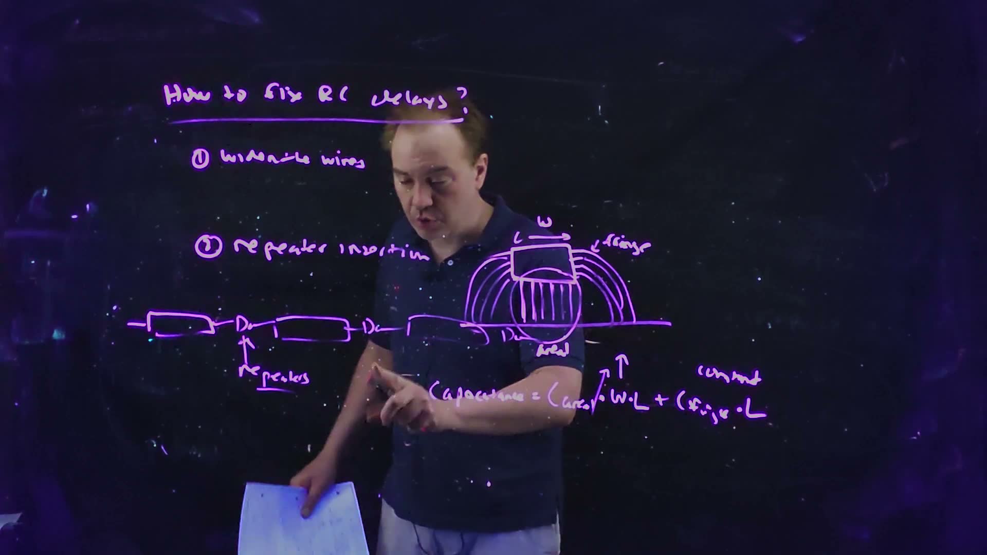
Fair copy of the board above (Lecture19 @ 52:02), mark for mark in its own layout. One pen (violet), copied in black. The board is the 49:19 board with the second fix added: “repeater insertion” after a ② rewritten lower, and the chain that cuts the wire into three pieces with a repeater (an inverter) after each. The third piece runs into the cross-section’s ground line, and its lower edge is faint; it is copied as far as drawn. The lecturer’s arm lies across “Capacitance = C_areal” in this frame; it is copied from 51:03. The capacitance line is levelled.

The wire part with k piecesadded

$$k\cdot\tfrac12\,\mathcal{R}\mathcal{C}\left(\frac{L}{k}\right)^2 = \frac1k\cdot\tfrac12\,\mathcal{R}\mathcal{C}L^2$$

Holds when: the wire's own (intrinsic) delay only; each repeater's delay and the pieces' loads come on top (Chapter 21)

Memorize or derive. Derive it in one line, as above.

A worked example added. The lecture’s wire, 3 mm long. Unbroken, its intrinsic delay is $9.5 \times 3^2 = 85.5$ ps. In three 1 mm pieces it is $3 \times 9.5 = 28.5$ ps of wire delay, before the two repeaters’ own delays, which Chapter 21 adds.

Check. Another route: per piece of length $L_p$ the wire part is $9.5\ \text{ps}\cdot(L_p/\text{mm})^2$(Lp​/mm)2, and there are $L/L_p$ pieces, so the total is $9.5\ \text{ps}\cdot(L/\text{mm})(L_p/\text{mm})$(L/mm)(Lp​/mm): linear in $L$ for a fixed piece length. With $L = 3$ mm and $L_p = 1$ mm that is $9.5 \times 3 \times 1 = 28.5$ ps ✓.

Trap. Counting only the saving. The repeaters’ delays and the loads they put on each piece come back in; only Chapter 21’s optimum says how many repeaters are worth it.

Check yourself For the same 3 mm wire, how many equal pieces keep the wire part of the delay under 10 ps, and how long is each?

The wire part is $85.5/k$ ps, so $k > 8.55$8.55: nine pieces, each $3000/9 = 333$ µm long, for $85.5/9 = 9.5$ ps. By the per-piece route: $9.5 \times 3 \times 0.333 = 9.5$ ps ✓. (Eight pieces give 10.69 ps.)

Check yourself Cut the 3 mm wire into four pieces instead of three. What is the wire part of the delay, and how much less is it than with three pieces?

$85.5/4 = 21.375$ ps, which is $28.5 - 21.375 = 7.125$ ps less, paid for with one more repeater.

10. Wire tapering

You need

The segment form (Section 7). Along the path to the receiver, each segment $k$ contributes $R_k(\tfrac12C_k + C_{down,k})$Cdown,k​): its resistance carries its own capacitance at half weight and everything beyond it.

The segment form: $R_k$ carries $\tfrac12C_k + C_{down,k}$Cdown,k​. Original figure ↑

Widening (Section 8). $\mathcal{R} = R_\square/W$ falls with width while $\mathcal{C} = C_{areal}W + C_{fringe}$ rises.

The areal and fringe parts (Lecture19 @ 49:19, redrawn): $C = C_{areal}WL + C_{fringe}L$Cfringe​L. Original figure ↑

The question. Widening a wire uniformly spends its width everywhere. Is the width worth more near the driver or near the receiver?

Wide near the driver (board, 52:18–54:56)

1. Two tapers. Draw a wire that is wide at the driver and narrows in steps towards the receiver, and one that does the opposite (52:53–53:21) board. “Should I widen the wire closer to the driver or … closer to the receiver?”
2. The Elmore weighting decides. Resistance near the driver counts against every capacitance beyond it; capacitance near the receiver counts against every resistance before it. So the driver end wants low resistance, and the receiver end wants low capacitance: wide, then narrow (53:23–54:30). “This scenario would be much better than this one” board.
3. Two segments added. With the segment form, a wire of two widths (near segment 1, far segment 2) into $C_{load}$ is $T = \tfrac12R_1C_1 + R_1(C_2 + C_{load}) + \tfrac12R_2C_2 + R_2C_{load}.$ Narrowing the far segment cuts $C_2$C2​, which $R_1$ sees in full; but it raises $R_2$R2​, which multiplies $C_{load}$ and half of $C_2$C2​. So $R_1C_2$ falls while $R_2C_{load}$ rises, and $\tfrac12R_2C_2$ rises too unless the capacitance is all areal ($R_2$R2​ grows as $1/W$1/W, the fringe part of $C_2$ does not shrink): in the example below it goes from 12.825 to 21.375 ps.
4. When it wins added. So tapering pays while the load is small next to the wire’s own capacitance. With the constants of Section 8, take a 3 mm wire in two 1.5 mm halves. Into a 20 fF load: uniform 2 µm, 53.58 ps; tapered 2 → 0.4 µm, 49.59 ps, faster with a third less capacitance (600 against 900 fF); the opposite taper, 169.29 ps. Into a 500 fF load the taper loses, 213.75 against 108.30 ps: the narrow far half’s resistance now works against a large load.
5. In practice. Tapering also saves routing and total capacitance, and “some of the routers actually support this idea of wire tapering” (54:56).

Wire tapering, redrawn from the board (Lecture19 @ 55:29). Top (✓): wide near the driver, narrow near the receiver. Bottom (✗): the opposite. The board circles the first and crosses out the second.

The board (Lecture19 @ 55:29)

Lecture19 @ 55:29Wire tapering: wide near the driver (circled), not the other way round (crossed out).

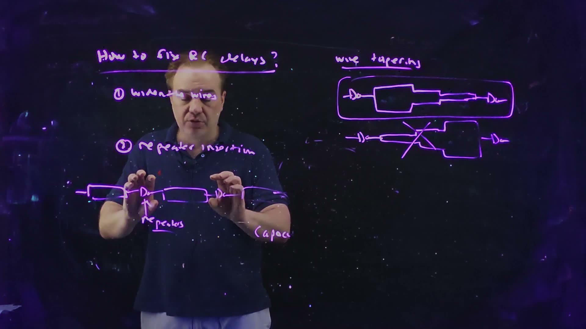
Fair copy of the board above (Lecture19 @ 55:29), mark for mark in its own layout. One pen (violet), copied in black. The loop marks the good taper, widest at the driver; the X strikes out the opposite taper, widest at the receiver. The left half is what is left of the 52:02 board after the cross-section and the capacitance line were erased: most of the third wire piece, its repeater and all but “Capac” of the capacitance line are gone. The lecturer’s hands and head cover the chain and “widen the wires” in this frame; the left half is copied from 54:30, which shows it clear and unchanged.

Tapering a 3 mm wire in two 1.5 mm halves added, computed from the two-segment Elmore sum with Section 8’s constants ($R_\square = 0.076$R□​= Ω/□, $C_{fringe} = 0.05$ fF/µm, $C_{areal} = 0.125$ fF/µm²). Widths in µm, driver end first; “W = 1.2” uses the same metal as the taper. With a 20 fF load (left) the taper is the fastest; with 500 fF (right) the uniform 2 µm wire is. The wires’ capacitances are 900, 600, 600 and 600 fF.

Two segments in seriesadded

$$T = \tfrac12R_1C_1 + R_1(C_2 + C_{load}) + \tfrac12R_2C_2 + R_2C_{load}$$

Holds when: two uniform segments (near 1, far 2) into a lumped load; the segment form of Section 7

Memorize or derive. Memorize the direction: wide near the driver, narrow near the receiver, while the load is small next to the wire. Derive the two-segment sum from the segment form: $R_1$ carries half of $C_1$ and everything beyond it, $C_2 + C_{load}$Cload​; $R_2$ carries half of $C_2$ and $C_{load}$Cload​.

A worked example added: the 20 fF case, term by term. Each half is 1500 µm.

Uniform 2 µm against a 2 → 0.4 µm taper, into 20 fF

1. The segments. At 2 µm: $R = 0.076 \times 1500/2 = 57\ \Omega$57 Ω, $C = (0.125 \times 2 + 0.05) \times 1500 = 450$ fF. At 0.4 µm: $R = 0.076 \times 1500/0.4 = 285\ \Omega$285 Ω, $C = 0.1 \times 1500 = 150$ fF.
2. Uniform 2 µm. $\tfrac12 \cdot 57 \cdot 450 = 12.825$ ps; $57 \times (450 + 20) = 26.79$ ps; $\tfrac12 \cdot 57 \cdot 450 = 12.825$ ps; $57 \times 20 = 1.14$ ps. Total 53.58 ps.
3. Taper 2 → 0.4 µm. $\tfrac12 \cdot 57 \cdot 450 = 12.825$ ps; $57 \times (150 + 20) = 9.69$ ps; $\tfrac12 \cdot 285 \cdot 150 = 21.375$ ps; $285 \times 20 = 5.7$ ps. Total 49.59 ps.
4. Why. The far half’s own terms cost the taper 13.11 ps more ($21.375 + 5.7$21.375+ against $12.825 + 1.14$1.14), but $R_1(C_2 + C_{load})$ saves it 17.1 ps, because the far half’s capacitance drops from 450 to 150 fF. The net gain is 3.99 ps.

Check. The first term is the same in both (the same near half) ✓. The opposite taper (0.4 µm near the driver) has $R_1 = 285\ \Omega$ in front of $450 + 20$ fF: $285 \times 470 = 133.95$ ps for that term alone, already worse than either wire above.

Traps.

• Tapering the wrong way, narrow at the driver: the narrow segment’s resistance then multiplies the whole wire.
• Assuming a taper always wins. With a large receiver load the far end needs low resistance too: 213.75 against 108.30 ps into 500 fF.
• Using one uniform-line formula for a tapered wire. Two widths are two segments.

Check yourself In the two-segment sum, which term carries the near segment's resistance against the far segment's capacitance?

$R_1C_2$R1​C2​, inside $R_1(C_2 + C_{load})$Cload​).

Check yourself Into 20 fF, compare the taper with a uniform 1.2 µm wire, which uses the same metal area. Which is faster, and by how much?

At 1.2 µm each half has $R = 0.076 \times 1500/1.2 = 95\ \Omega$ and $C = (0.125 \times 1.2 + 0.05) \times 1500 = 300$ fF. Term by term: $\tfrac12 \cdot 95 \cdot 300 = 14.25$ ps; $95 \times (300 + 20) = 30.4$ ps; $14.25$ ps; $95 \times 20 = 1.9$ ps; total 60.80 ps. The taper takes 49.59 ps, so it is faster by 11.21 ps with the same metal.

On the exam

Wires are on all four past finals, 99 points in all, usually as a wire drawing with lengths, a sheet resistance and a capacitance per micron (FN12-9’s wire is straight, and FN17-3 gives the resistance per micron directly). The practice page for interconnect, FW1, solves these parts; this chapter teaches the methods and solves none of them.

Part	Points	What it asks	Sections
FN10-8a	10	Elmore delay from A to one receiver of a branching wire, 100 fF at each receiver	§7, §4
FN10-8b	10	the same, with 200 fF added 1000 µm before each receiver	§7
FN12-9a	10	Elmore delay of a 4000 µm point-to-point wire into 30 fF, with $C$ given as a function of $W$	§4, §5, §8
FN12-9b	10	the same wire widened from 0.4 to 4 µm	§8
FN12-9c	12	the first half 4 µm, the second 0.4 µm: compare, and say why tapering helps	§10, §7
FN19-7a	8	why the capacitance per length has the form $0.04 + 0.15W$	§8
FN19-7b	10	Elmore delay from A to B of a branching wire	§7, §8
FN19-7c	8	with an FO1 delay of 50 ps, must resistance be considered?	§6
FN19-7d	10	the trunk widened from 0.4 to 10 µm: the new delay	§7, §8, §10
FN17-3a	11	a clock tree: the total delay from A to B, buffers plus Elmore wires	§7, §6 (and Chapter 7’s gate delay)

A note on FN19-7. The paper prints the width as “0.4 mm” on its first page and “0.4 µm” in part (d). Read it as 0.4 µm: part (d) widens “from 0.4 µm”, and FN10-8 is the same tree at 0.4 µm.

A note on FN17-3. The clock tree is the one setup here with several levels of branching, and its key has inconsistent intermediate values. Its delay from A to B has three pieces, each from this chapter or Chapter 7:

1. The root buffer drives the whole tree’s capacitance, every wire and every leaf buffer’s input: Chapter 7’s $\tau_{inv}\,C_{load}/C_{in}$τinv​Cload​/Cin​, with no resistive shielding, as the paper says (Section 6).
2. The wire’s Elmore delay from the root buffer’s output to the input of B’s leaf buffer, over the path’s five segments by the segment form (Section 7): at each branch node, the subtrees that leave the path are side branches, lumped there with their wires and their leaf buffers’ input capacitance, so each segment’s $C_{down,k}$ nests inside the one before. The half of the tree that leaves at the driver node itself shares no resistance with the path, so it adds nothing here: it only loads the root buffer in piece 1.
3. The leaf buffer drives B’s 500 fF: $\tau_{inv}\,C_{load}/C_{in}$ again.

The practice page settles the numbers. Parts (b) and (c), jitter and inductance, are Chapter 21’s.

Memorize.

• $R = R_\square L/W$R□​L/W; $\mathcal{R} = R_\square/W$R□​/W; about 0.1 fF/µm; upper levels have lower $R_\square$R□​.
• The Elmore rule: every capacitance times the resistance it shares with the path to the receiver. Intrinsic and extrinsic parts.
• $T_{Elmore} = \tfrac12\mathcal{R}\mathcal{C}L^2 + \mathcal{R}L\,C_{load}$RLCload​, quoted as the delay (no ln 2).
• Delay ≈ $T_{Elmore}$TElmore​; slew degradation ≈ $2T_{Elmore}$2TElmore​. Resistance matters when $T_{Elmore}$ is comparable to the slew or larger.
• Side branches are lumped at the node where they leave the path.
• $C = C_{areal}WL + C_{fringe}L$Cfringe​L: widening always helps the extrinsic part, the intrinsic part only in its fringe share.
• Tapers go wide near the driver, narrow near the receiver, and win while the load is small next to the wire.

Derive (with the path).

• The ½. A slice at $x$ sees $\mathcal{R}x$Rx; $\int_0^L \mathcal{R}x\,\mathcal{C}\,dx = \tfrac12\mathcal{R}\mathcal{C}L^2$21​RCL2; or $k$ sections, $(k+1)/(2k) \to \tfrac12$21​.
• The segment form. Collect each path resistor’s terms: $R_k(\tfrac12C_k + C_{down,k})$Cdown,k​), summed along the path.
• Widening. Substitute $\mathcal{R} = R_\square/W$ and $\mathcal{C} = C_{areal}W + C_{fringe}$Cfringe​: $\tfrac12R_\square(C_{areal} + C_{fringe}/W)L^2 + (R_\square/W)LC_{load}$(R□​/W)LCload​.
• Two segments. $\tfrac12R_1C_1 + R_1(C_2 + C_{load}) + \tfrac12R_2C_2 + R_2C_{load}$R2​Cload​.
• Scaling. $C \sim s_L$sL​, $R \sim s_Ls^2$sL​s2, $RC \sim s_L^2s^2$sL2​s2.

Method card. The playbook’s card for Elmore wires: per-length values first, then the path’s segments, each segment’s $R_k(\tfrac12C_k + C_{down,k})$Cdown,k​), the sum, and a comparison with the technology’s edges.

All the boards of Lecture 19 (20 frames)

Lecture19 @ 01:41 wires: capacitance, resistance, inductance; capacitance ⇒ 0.…

Lecture19 @ 05:15 R = (ρ/t)(L/W); sheet resistance; L/W squares; lower level 0.04 Ω/□

Lecture19 @ 07:37 upper levels; Cu BEOL and the liner

Lecture19 @ 12:32 scaling: C ∼ s_L, R ∼ s_L s², RC ∼ s²

Lecture19 @ 13:45 scaling, with s² circled

Lecture19 @ 20:16 Elmore delay: the wire and its ladder; Padé

Lecture19 @ 24:23 the Elmore sum; intrinsic and extrinsic

Lecture19 @ 24:39 the single-pole receiver model

Lecture19 @ 27:59 the uniform line: ½ℛ𝒞L² + ℛL·C_load

Lecture19 @ 31:12 when does resistance matter? slew rate ⇔ Elmore delay

Lecture19 @ 33:54 resistive shielding; the π model

Lecture19 @ 37:59 two Elmore delays; the side-branch sum begun

Lecture19 @ 39:26 A→B with the side branch lumped

Lecture19 @ 40:46 the worked example: the givens

Lecture19 @ 45:26 the worked example: 9.5 + 95 = 104.5 ps

Lecture19 @ 47:40 how to fix RC delays: widen the wires

Lecture19 @ 49:19 areal and fringe capacitance

Lecture19 @ 52:02 repeater insertion

Lecture19 @ 54:30 wire tapering

Lecture19 @ 55:29 wire tapering: the good and the bad taper