7. Delay models and static CMOS gates

Lecture 6 described how an inverter switches: a curved trajectory across the I–V curves, a 50% delay, a slew. That picture is accurate but far too slow to use for every gate on a chip. Lecture 7 replaces it with the model designers actually use for quick estimates: every transistor is a “resistance” that shrinks with its width, every gate input is a capacitance that grows with its width, and delay is one times the other. The lecture shows how to measure the two numbers for a technology, then builds the logic gates beyond the inverter (static CMOS: NOR, NAND, AOI), and finally uses the model to compare them. The comparison gives the lecture’s last and most important idea: a NAND or NOR is slower than an inverter of the same strength by a fixed factor, its logical effort.

After this chapter you can:

1. explain the simplified delay model and why its “resistance” is really a constant of proportionality between load and delay;
2. use $C_g$ in fF/µm and $R_{nfet}$Rnfet​, $R_{pfet}$ in kΩ·µm to compute the delay of any transistor driving any load;
3. describe the two fan-out-of-four simulations that measure $C_g$ and $R$R, and say why drain capacitance must be zeroed in one of them;
4. state what makes a gate static CMOS, build complementary NOR, NAND and AOI gates as duals, and check their truth tables;
5. explain pin swapping, why tall stacks are avoided, and how a static gate can be non-complementary;
6. derive $\mathrm{FO1} = 3R_{nfet}C_g = \tau_{inv}$τinv​, size a stack for equal drive, and find the logical effort of NAND (4/3) and NOR (5/3);
7. write a gate’s delay as its gain $g \cdot h$ times $\tau_{inv}$τinv​.

Boxes and equations marked board were written in the lecture. Parts marked added are explanations or examples this guide adds.

Before you start

You need these ideas from earlier chapters. Each is restated here.

• Gate capacitance (Chapters 4 and 5). A transistor’s gate is a capacitor of area $WL$ with $C_{ox} = \kappa_{ox}\varepsilon_0/t_{ox}$ per unit area, so $C_{gate} = WLC_{ox}$WLCox​.
• Current grows with width (Chapter 4). Every I–V model has $I_D \propto W$W. Twice the width carries twice the current, so it charges a load in half the time.
• PFETs are weaker (Chapter 5). Holes are slower than electrons, so a PFET delivers about half the current of an NFET of the same width. An inverter’s PFET is made twice as wide ($2W$2W against $W$W) for equal rise and fall.
• FO1 and FO4 (Chapter 5). The delay of an inverter driving one copy of itself (fan-out of one), or four copies (fan-out of four).
• Delay and slew (Chapter 6). Delay is measured from the input’s 50% point to the output’s: $t_{pHL}$ for a falling output, $t_{pLH}$ for a rising one. A saturated ramp is a waveform that is flat, ramps linearly, and is flat again.

Notation. $W_n$ and $W_p$ are the NFET and PFET widths. A sizing written “16/8” means a PFET 16 µm wide and an NFET 8 µm wide, as on the lecture’s boards; “4(16/8)” means four times that, 64/32. The board writes $R_{nfet}$ and $R_{pfet}$Rpfet​; this chapter writes them the same way. $\tau_{inv}$ is the FO1 delay (Section 7).

1. From trajectories to a simple delay model

The idea. Treat the pull-up and pull-down as a switch with a resistor, so that every delay is a “resistance” times the capacitance being driven.

Lecture07 @ 04:21The real trajectory and its straight-line replacement (centre), the output waveform (right), and the switch-and-resistor model (left).

The trajectory, once more

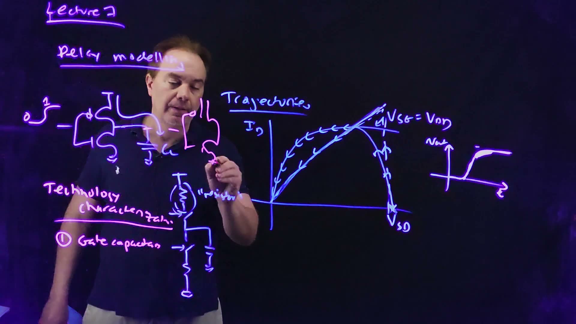
The lecture starts where Lecture 6 ended (00:25). An inverter’s input switches from $V_{DD}$ to 0, and its PFET charges the load. On the PFET’s I–V curves the operating point rises quickly to the full-overdrive curve, $V_{SG} = V_{DD}$VDD​, then rides that curve down (01:10). The output rises almost linearly at first, then slows into a tail as the PFET leaves saturation for triode (01:41). Lecture 6 called this the trajectory.

The simplified picture

Since the 1980s, designers have used a much simpler picture (02:09) board:

• each pull-up and pull-down network is a switch in series with a resistor;
• switching the input closes one switch, and the load charges (or discharges) through that resistor;
• on the I–V plane, the curved trajectory becomes a straight line: an immediate jump up, then charging along a resistor’s line (02:39).

A constant of proportionality, not a resistor

The lecturer is careful about the word (03:09). The “resistor” is not a real resistor in the circuit. It is a constant of proportionality between capacitance and delay, measured for each technology:

$$t_{delay} = R \times C_{load}.$$

The delay is linear in the load, and the constant has the units of resistance (03:29). Since it is measured as delay ÷ capacitance, it already contains whatever factors the real waveform has.

Units. added $1\,\mathrm{k\Omega} \times 1\,\mathrm{fF} = 10^3 \times 10^{-15}\,\mathrm{s} = 1\,\mathrm{ps}$1ps. With $R$ in kΩ and $C$ in fF, the delay comes out in picoseconds directly.

Common mistakes.

• Multiplying by $\ln 2 \approx 0.69$0.69. added For a real resistor and capacitor, the 50% point comes at $0.69RC$0.69RC. Here $R$ is defined as measured delay ÷ load, so $t = RC$ already is the 50% delay; multiplying again by 0.69 gets the measurement wrong.
• Thinking the model describes the waveform. It predicts one number, the delay, and nothing about the shape.

2. Characterizing a technology: gate capacitance and resistance

The idea. Two numbers per technology are enough: the gate capacitance per micron of width, and the “resistance” times micron of width for each kind of transistor.

Lecture07 @ 09:32The two technology numbers: C_g in fF/µm (centre) and R_nfet, R_pfet in kΩ·µm, divided by the device width (right).

Number one: gate capacitance per micron

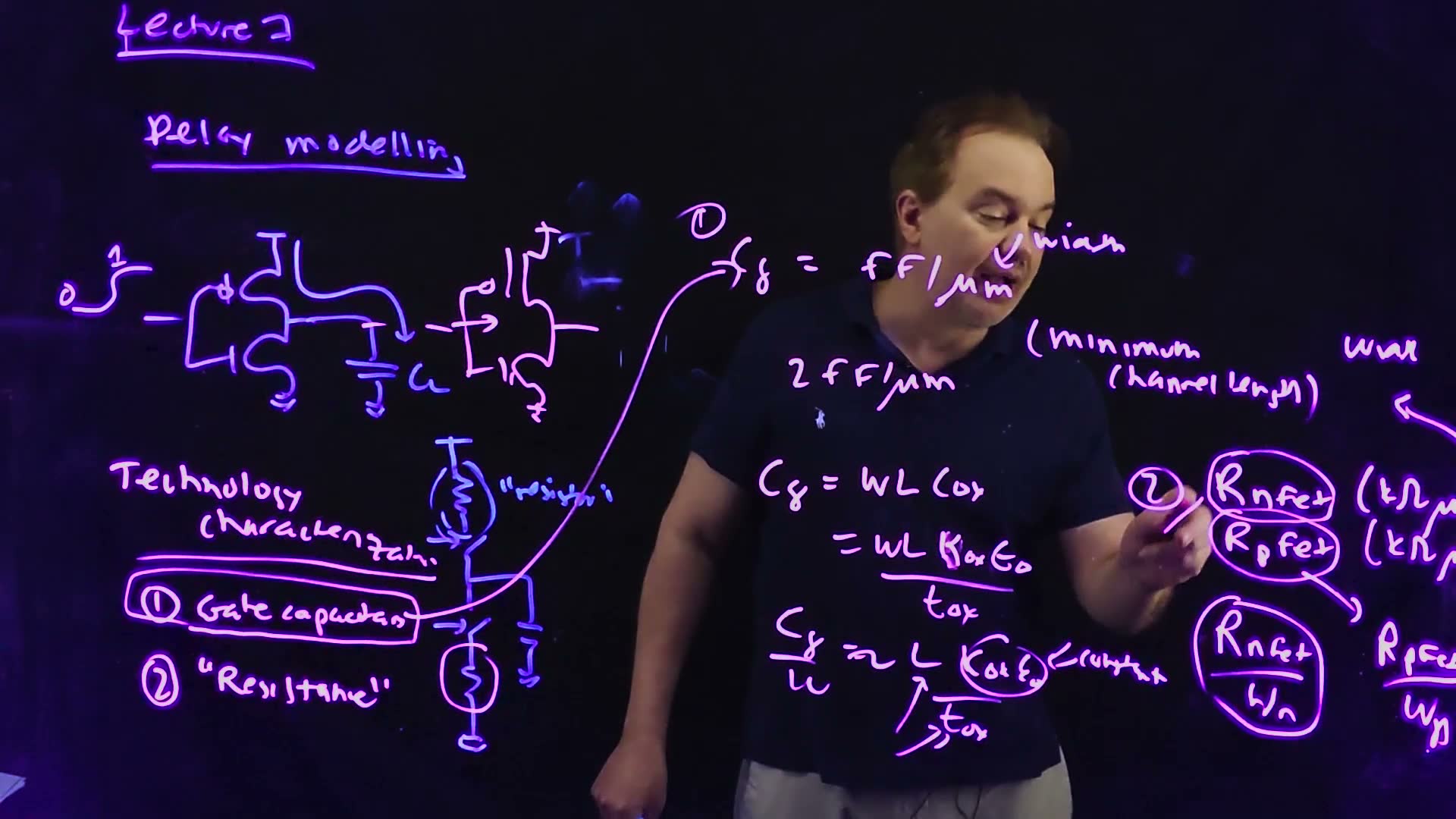
When one inverter drives another, what capacitance does it see looking into the second one’s input (04:15)? The lecture characterizes it as femtofarads per micron of device width, $C_g$ in fF/µm, for a minimum-length device, because almost every logic transistor is minimum length (05:03–05:30) board.

• The number is about 2 fF/µm board, essentially the same for NFETs and PFETs (05:58).
• It has stayed near 2 fF/µm for many technology generations. Recently it has drifted a little, and the problem set’s 90 nm technology gives a slightly different value (06:00).

Why it hardly changes (06:15–07:32):

Gate capacitance per micron of width (board, 06:15–07:32)

1. The gate is a capacitor of area $WL$ board: $C_g = WLC_{ox}$WLCox​.
2. With the oxide capacitance written out board: $C_g = WL\,\dfrac{\kappa_{ox}\varepsilon_0}{t_{ox}}$WLtox​κox​ε0​​. (The lecturer starts to say “epsilon ox” and corrects himself to $\kappa_{ox}$κox​, the oxide’s dielectric constant.)
3. Divide by the width board: $\dfrac{C_g}{W} = L\,\dfrac{\kappa_{ox}\varepsilon_0}{t_{ox}}$Ltox​κox​ε0​​. The factor $\kappa_{ox}\varepsilon_0$ is a constant.
4. Under Dennard scaling (Chapter 4), $L$ and $t_{ox}$ both shrink by the same factor $\kappa$κ. Their ratio $L/t_{ox}$ doesn’t change, so neither does $C_g/W$ (07:06).

Worked example. added Chapter 4’s device, $t_{ox} = 5.4\,\mathrm{nm}$ and $L = 0.25\,\mu\mathrm{m}$0.25μm:

1. $C_{ox} = \dfrac{3.9 \times 8.854\times10^{-14}\,\mathrm{F/cm}}{5.4\times10^{-7}\,\mathrm{cm}} = 6.39\times10^{-7}\,\mathrm{F/cm^2}$10−7F/cm2.
2. Convert: $1\,\mathrm{F/cm^2} = 10^{15}\,\mathrm{fF}/10^{8}\,\mu\mathrm{m^2} = 10^{7}\,\mathrm{fF/\mu m^2}$107fF/μm2, so $C_{ox} = 6.39\,\mathrm{fF/\mu m^2}$6.39fF/μm2.
3. $C_g/W = L\,C_{ox} = 0.25\,\mu\mathrm{m} \times 6.39\,\mathrm{fF/\mu m^2} = 1.60\,\mathrm{fF/\mu m}$1.60fF/μm: close to the lecture’s 2 fF/µm.
4. Scale by $\kappa = 2$2: $L = 0.125\,\mu\mathrm{m}$0.125μm, $t_{ox} = 2.7\,\mathrm{nm}$2.7nm. $C_{ox}$ doubles and $L$ halves, so $C_g/W$ is still 1.60 fF/µm.

Loads as widths. added Since every gate input is $C_g$ per micron, a load can be written as an equivalent gate width, $C/C_g$C/Cg​. At 2 fF/µm, a 50 fF load “is” 25 µm of gate. Past exams use this often.

Number two: resistance times micron

The second number is the “resistance” of each kind of transistor, in kΩ·µm, where the micron is again the channel width (08:05) board. There is one value for the NFET and one for the PFET:

• divide by the actual width to get that device’s resistance: $R_{nfet}/W_n$ and $R_{pfet}/W_p$ (08:24) board;
• multiply by the load to get the delay of discharging (NFET) or charging (PFET) it (08:49).

A PFET has half the current drive of an NFET, so a characterized technology should show $R_{pfet} \approx 2R_{nfet}$ (09:20).

The simplified delay modelboard

$$t_{pHL} = \frac{R_{nfet}}{W_n}\,C_{load}$$$$t_{pLH} = \frac{R_{pfet}}{W_p}\,C_{load}$$$$C_{gate} = C_g\,(W_n + W_p)$$$$R_{pfet} \approx 2R_{nfet}$$

$C_g \approx 2\,\mathrm{fF/\mu m}$ and roughly constant across generations ($C_g/W = L\kappa_{ox}\varepsilon_0/t_{ox}$Cg​/W=Lκox​ε0​/tox​). The input capacitance of an inverter, $C_g(W_n + W_p)$Wp​), is the board’s “gate capacitance looking into this inverter” written out.

Holds when: minimum-length devices; C_g in fF/µm of gate width; R in kΩ·µm; gate loading only, drain capacitance ignored (Section 3)

Worked example. added A technology with $R_{nfet} = 2\,\mathrm{k\Omega\cdot\mu m}$ and $R_{pfet} = 4\,\mathrm{k\Omega\cdot\mu m}$4kΩ⋅μm; an inverter with an 8 µm PFET and a 4 µm NFET drives 20 fF.

1. NFET: $R_{nfet}/W_n = 2/4 = 0.5\,\mathrm{k\Omega}$0.5kΩ, so $t_{pHL} = 0.5 \times 20 = 10\,\mathrm{ps}$10ps.
2. PFET: $R_{pfet}/W_p = 4/8 = 0.5\,\mathrm{k\Omega}$0.5kΩ, so $t_{pLH} = 0.5 \times 20 = 10\,\mathrm{ps}$10ps.
3. Equal: the 2:1 width ratio exactly cancels the 2:1 resistance ratio. That is why inverters are sized $2W/W$2W/W.

Check yourself An NFET 2 µm wide, in a technology with R_nfet = 2.5 kΩ·µm and C_g = 2 fF/µm, discharges a load equal to 12 µm of gate. What is the delay?

The load is $12\,\mu\mathrm{m} \times 2\,\mathrm{fF/\mu m} = 24\,\mathrm{fF}$24fF. The NFET’s resistance is $2.5/2 = 1.25\,\mathrm{k\Omega}$1.25kΩ. Delay $= 1.25 \times 24 = 30\,\mathrm{ps}$30ps.

3. Measuring the two numbers in simulation

The idea. Both numbers come from fan-out-of-four simulations with the technology’s SPICE models: first match a plain capacitor to a gate’s load to find $C_g$Cg​, then time an inverter driving a known gate load to find $R$R.

When you get a new technology’s models, you run a few circuit simulations to find $C_g$Cg​, $R_{nfet}$ and $R_{pfet}$ (09:20). The lecture describes the two set-ups you will build in problem set 3, for its 90 nm technology (10:01, 25:26).

Lecture07 @ 18:15The capacitance bench: match C_L to the 8(16/8) inverter's input, then C_g = C_L/(8(16 + 8) µm).

Bench 1: gate capacitance

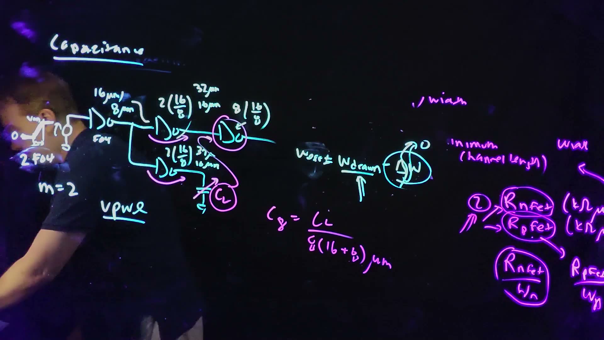
The circuit (10:49–14:23) board:

1. A first inverter of 16/8. The lecturer picks “something relatively beefy” on purpose (11:03). The width a transistor really has is the drawn width minus a correction, $W_{eff} = W_{drawn} - \Delta W$ board, and for very narrow devices $\Delta W$ matters. Wide devices make it negligible (11:30–12:32). (He says “let me just make it 10 by 8” at 12:32; the board, and his words before and after, say 16 by 8.)
2. It drives two inverters of 2(16/8): a 32 µm PFET and a 16 µm NFET each. Together they are four times its own size, a fan-out of four (12:32). In the schematic you can type 32 and 16, or type 16 and 8 and set the multiplier $m = 2$2, two devices in parallel (13:26).
3. The upper 2(16/8) drives an inverter of 8(16/8), four times its size: fan-out of four again (14:03).
4. The lower 2(16/8) drives a plain capacitor $C_L$CL​.

The input is a saturated ramp from 0 to $V_{DD}$VDD​, entered with the VPWL source (14:32). Its slew time is set to about twice the FO4 delay, which you measure separately: that is roughly the slew of a real gate loaded at fan-out of four (15:06–15:27). The ramp is still too abrupt to be realistic, so the first inverter’s job is to clean it up into a genuine FO4 waveform (16:00).

The measurement (16:32–17:51). Vary $C_L$ until the two 2(16/8) inverters have equal delays, rising or falling, it doesn’t matter. Then $C_L$ is the input capacitance of the 8(16/8) inverter, whose gates total $8 \times (16 + 8)\,\mu\mathrm{m}$ board:

$$C_g = \frac{C_L}{8\,(16 + 8)\,\mu\mathrm{m}}.$$

Bench 2: resistance

Lecture07 @ 24:54The resistance bench: R_nfet = t_pHL/C_L × 4(8 µm), R_pfet = t_pLH/C_L × 4(16 µm), with drain capacitance zeroed (AS = AD = PS = PD = 0).

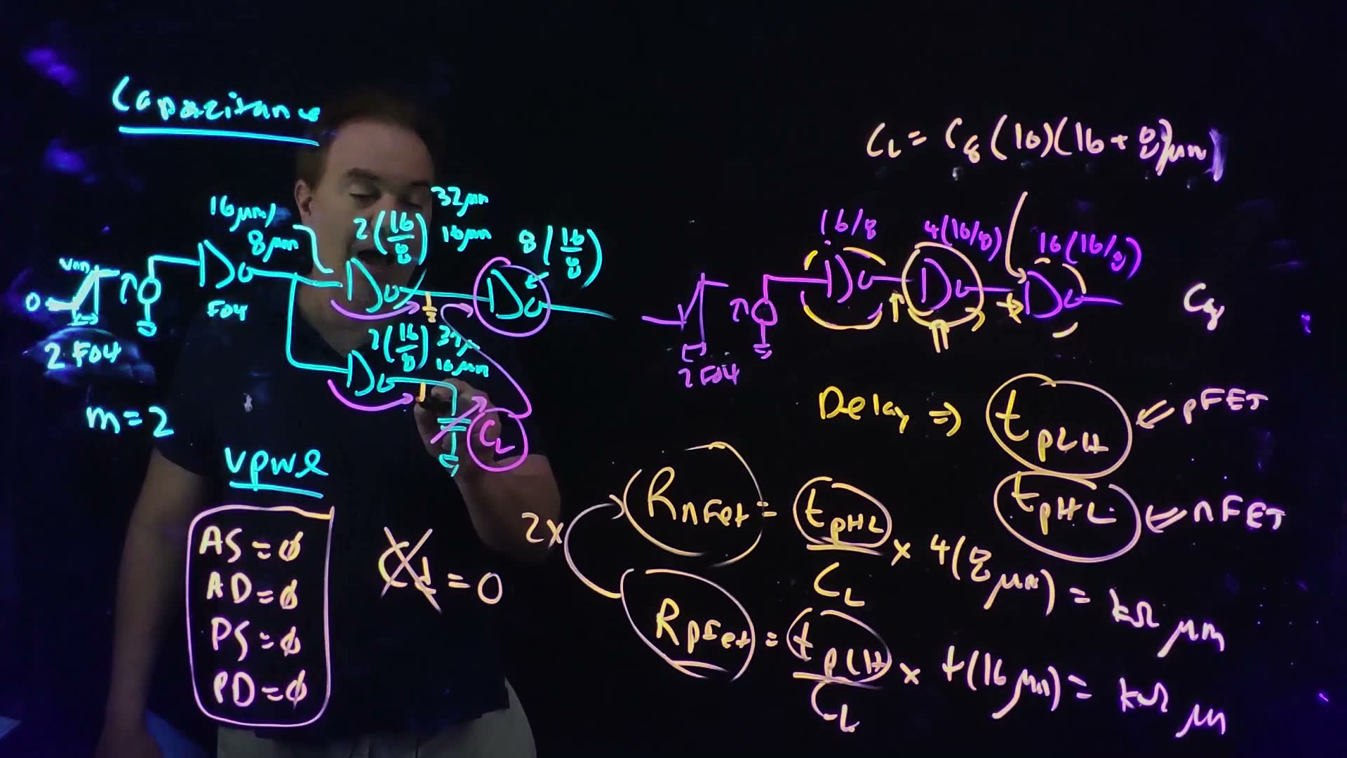
The circuit (18:36) board: three inverters in a row, 16/8, 4(16/8) and 16(16/8), each at fan-out of four, driven by the same kind of ramp. The first cleans up the waveform; the last provides a realistic load; the one being measured is the middle one (19:09).

Measure its two delays (19:38–20:06) board: $t_{pLH}$ characterizes the PFET (pull-up), $t_{pHL}$ the NFET (pull-down).

R from the middle inverter (board, 20:06–22:23)

1. The load is the last inverter’s input board: $C_L = C_g \times 16 \times (16 + 8)\,\mu\mathrm{m}$8)μm, using the $C_g$ from bench 1.
2. Delay ÷ load gives the NFET’s resistance in kΩ; multiply by its width, $4 \times 8\,\mu\mathrm{m}$ board: $R_{nfet} = \dfrac{t_{pHL}}{C_L} \times 4(8\,\mu\mathrm{m})$4(8μm), in kΩ·µm.
3. The same for the PFET, width $4 \times 16\,\mu\mathrm{m}$ board: $R_{pfet} = \dfrac{t_{pLH}}{C_L} \times 4(16\,\mu\mathrm{m})$4(16μm).
4. The inverter is sized 2:1 for equal pull-up and pull-down, so the two delays should be about equal, and then $R_{pfet}$ comes out twice $R_{nfet}$ board (21:40–22:23).

Zero the drain capacitance

This model’s only load is gate capacitance (22:30). Lecture 5 showed how important drain capacitance is, but the quick sizing methods that follow ignore it, and full circuit simulation corrects for it later (22:56). So the characterization must ignore it too.

• In Virtuoso’s instance properties, each transistor has four parameters describing its diffusions: AS and AD, the source and drain areas, and PS and PD, their perimeters (23:14). Setting all four to zero removes the junction capacitance, the main part of the drain capacitance board.
• It matters in bench 2: the middle inverter’s own drain capacitance would add to its load and make $R$ come out too large (24:56).
• It doesn’t matter in bench 1: both 2(16/8) inverters have the same drain capacitance, so it affects both delays equally and the match happens at the same $C_L$ (24:30).

Try both benches. Slide the capacitor until the two delays match, read off $C_g$Cg​, and watch the resistances underneath. Then switch the drain capacitance back on.

Technology 1Technology 2Drain caps zeroed (AS = AD = PS = PD = 0)

capacitor C_L in bench 1

120 fF

bench 1: delay into the 8(16/8) inverter

24.00 ps

bench 1: delay into C_L

15.00 ps

C_g = C_L/(8 × 24 µm)

0.625 fF/µm

bench 2: C_L = C_g × 16 × 24 µm

240.0 fF

bench 2: t_pHL, t_pLH measured

24.00, 24.00 ps

R_nfet = t_pHL/C_L × 32 µm

3.20 kΩ·µm

R_pfet = t_pLH/C_L × 64 µm

6.40 kΩ·µm

R_pfet/R_nfet

2.00

τ_inv = 3R_nfetC_g from these

6.00 ps

Not matched yet: the capacitor-loaded delay is shorter by 9.00 ps, so raise C_L. Until it matches, the C_g and both R values above are off.

Each technology hides its own C_g, R_nfet and R_pfet. Bench 1's two inverters have the same drain capacitance, so it cancels in the comparison: toggle it and the crossing doesn't move. In bench 2 nothing cancels it, which is why the lecture zeroes AS, AD, PS and PD there. Bench 2's delay is itself an FO4 delay, 4τ_inv, in this model. The delays here come from the simplified model, (R/W) × C, not from a circuit simulation, so the waveform-shaping first inverter and the input ramp of twice FO4 have no effect on them.

What to notice.

• Away from the match, the $C_g$ you read is wrong, and both resistances inherit the error: bench 2 divides by a load computed from your $C_g$Cg​.
• Turn the drain caps on: the crossing in bench 1 doesn’t move, but bench 2’s delays grow and both resistances come out 12.5% too large in Technology 1.
• Bench 2’s delay is an FO4 delay, and in this model it equals $4\tau_{inv}$ exactly (Section 7). added

Worked example. added Illustrative numbers, the widget’s Technology 1.

1. Bench 1 matches at $C_L = 192\,\mathrm{fF}$192fF: $C_g = 192/(8 \times 24) = 192/192 = 1.00\,\mathrm{fF/\mu m}$1.00fF/μm.
2. Bench 2’s load: $C_L = 1.00 \times 16 \times 24 = 384\,\mathrm{fF}$384fF.
3. Bench 2 measures $t_{pHL} = t_{pLH} = 24\,\mathrm{ps}$24ps.
4. $R_{nfet} = (24/384) \times 32 = 2.0\,\mathrm{k\Omega\cdot\mu m}$2.0kΩ⋅μm.
5. $R_{pfet} = (24/384) \times 64 = 4.0\,\mathrm{k\Omega\cdot\mu m}$4.0kΩ⋅μm: twice $R_{nfet}$Rnfet​, as expected.
6. Had the drain caps been left in, with $C_d = 0.5\,\mathrm{fF/\mu m}$ (Chapter 5’s $\eta = C_g/C_d = 2$2): the middle inverter adds $96\,\mu\mathrm{m} \times 0.5 = 48\,\mathrm{fF}$48fF, the delay becomes $(2/32) \times (384 + 48) = 27\,\mathrm{ps}$27ps, and the extraction gives $R_{nfet} = (27/384) \times 32 = 2.25\,\mathrm{k\Omega\cdot\mu m}$2.25kΩ⋅μm, 12.5% too high.

Common mistakes.

• Dividing by the wrong width. Bench 1 divides by the receiving inverter’s total gate width, $8 \times (16 + 8)$8). Bench 2 multiplies by the measured inverter’s NFET (or PFET) width, $4 \times 8$ (or $4 \times 16$16).
• Using $t_{pLH}$ for the NFET. A falling output is the NFET’s job: $t_{pHL}$ goes with $R_{nfet}$Rnfet​.
• Forgetting to zero AS, AD, PS, PD in bench 2.

Check yourself In bench 1 the two delays match at C_L = 150 fF. What is C_g? Bench 2 then gives t_pHL = 30 ps. What is R_nfet?

$C_g = 150/(8 \times 24) = 150/192 = 0.781\,\mathrm{fF/\mu m}$0.781fF/μm. Bench 2’s load is $0.781 \times 16 \times 24 = 300\,\mathrm{fF}$300fF, so $R_{nfet} = (30/300) \times 32 = 3.2\,\mathrm{k\Omega\cdot\mu m}$3.2kΩ⋅μm. (HW3-1 asks exactly this, with simulated numbers.)

Check yourself Why does bench 1 still give the right C_g if you forget to zero the drain capacitance, while bench 2 doesn't give the right R?

In bench 1 two identical inverters are compared, and each carries the same drain capacitance, so it adds the same delay to both and cancels in the comparison. In bench 2 the measured delay is divided by the gate load alone, so any drain capacitance is wrongly charged to the transistor’s resistance.

4. Static CMOS gates

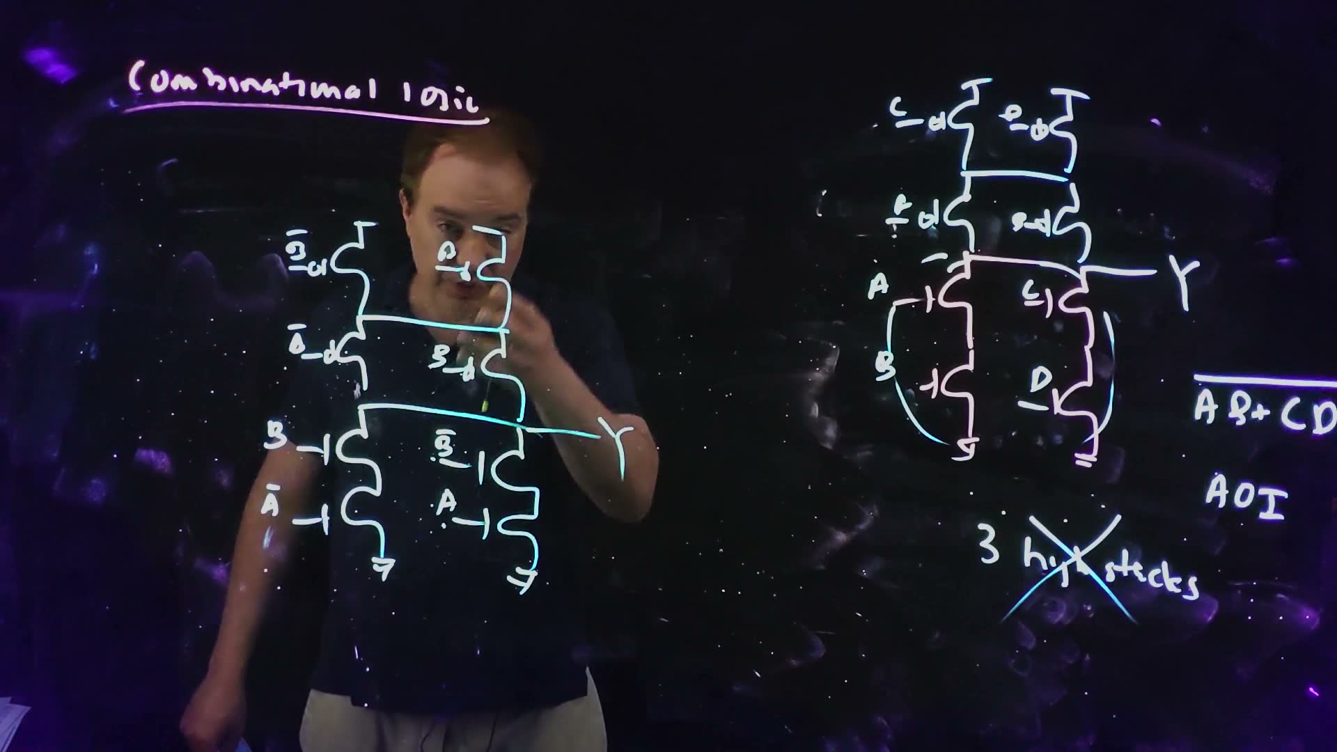
The idea. A static CMOS gate has a pull-up network of PFETs and a pull-down network of NFETs, and for any settled inputs exactly one of them is on. Making the two networks duals of each other guarantees it.

Lecture07 @ 31:52Static CMOS: a pull-up network of PFETs and a pull-down network of NFETs; complementary networks are duals (series ↔ parallel); the NOR and its truth table.

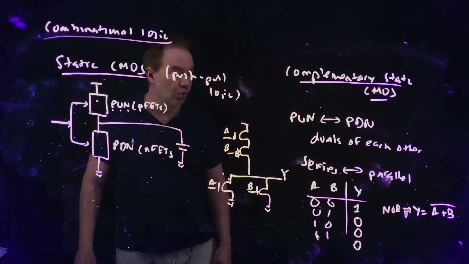
Why we need more than the inverter

So far the only gate is the inverter, and “obviously we can’t make a computer with an inverter”: it is not logically complete (25:54). We need general combinational gates; sequential elements (latches, flip-flops) come later (26:22).

What “static” means

The structure (27:13) board:

• a pull-up network (PUN) of PFETs between $V_{DD}$ and the output;
• a pull-down network (PDN) of NFETs between the output and ground;
• the load capacitance on the output.

The gate is static CMOS if, for every static set of inputs, exactly one network is on (27:44–28:15): either the pull-up connects the output to $V_{DD}$ or the pull-down connects it to ground. Never both, never neither. The other cases are other logic families, both taken up later (28:15):

• both on: ratioed logic;
• both off: dynamic logic.

Static CMOS is also called push-pull logic board: one network pushes the output up, the other pulls it down (28:44).

Complementary static CMOS: duals

The simplest way to guarantee the static condition is complementary static CMOS (28:56) board: the two networks are duals of each other. In terms of switches, wherever one network has a series connection, the other has a parallel one (29:41–30:01) board. Complementary always means static; static does not always mean complementary (29:16; Section 6 shows one).

The NOR (board, 30:01–31:56)

1. Pull-down: two NFETs, A and B, in parallel. The dual pull-up: two PFETs in series.
2. A = 0, B = 0: both NFETs off, so the pull-down is off; both PFETs on, so the pull-up is on. Y = 1.
3. A = 0, B = 1 (or A = 1, B = 0): one NFET is on, so the pull-down is on; one PFET is off, so the series pull-up is off. Y = 0.
4. A = 1, B = 1: Y = 0.
5. Y is 1 only when neither input is 1 board: $Y = \overline{A + B}$A+B​, a NOR.

Swap the roles (32:08): NFETs in series, PFETs in parallel. The pull-down conducts only when both inputs are 1, so $Y = \overline{AB}$AB, a NAND board. The lecturer leaves the truth table to you (32:39); the widget has it.

NORNANDAOIConstrained gate, dual pull-upConstrained gate, link removed

A = 0B = 0

pull-up network (PFETs)

on

pull-down network (NFETs)

off

output Y

1

Only the pull-up conducts: Y is connected to V_DD.

A	B	up	down	Y
0	0	on	–	1
0	1	on	–	1
1	0	on	–	1
1	1	–	on	0

Boxes are transistors, labelled with the input on their gate; a circle marks a PFET. Green boxes conduct. Series devices conduct only if all are on, parallel devices if any one is. The gates are drawn as switch networks, not as layouts, and sizes are left out (Section 8 sizes them). "Set all four inputs freely" is added: it breaks the constraint Ā = NOT A, B̄ = NOT B, to show why the link can only be removed when the constraint holds.

What to notice.

• For every input combination of NOR, NAND and AOI, exactly one network is green: the readout never says “contention” or “floating”. That is what “static” means.
• Series devices conduct only if all are on; parallel devices if any one is. The pull-up of a NOR is a series stack, so it conducts only for A = B = 0.

Check yourself Write the truth table of the two-input NAND and say which network is on in each row.

A = 0, B = 0: both parallel PFETs on, series NFETs off, Y = 1. A = 0, B = 1 and A = 1, B = 0: one PFET on (enough, they are in parallel), the series NFETs off, Y = 1. A = 1, B = 1: both PFETs off, both NFETs on, Y = 0. Exactly one network conducts in every row, so the gate is static.

Check yourself A gate's pull-up and pull-down are both on for one input combination. Is it static CMOS? What happens to the output?

No. Static CMOS needs exactly one network on. With both on, the output is a contest between the two networks, the situation the lecture calls ratioed logic (28:15); the output settles somewhere between the rails, set by their relative strengths.

5. Pin swapping, AOI gates and the stack limit

The idea. Gates with series stacks can be built in more complex forms, but each stacked device makes the gate slower. The device nearest the output is the fastest, and stacks taller than about three are avoided.

Lecture07 @ 34:56NAND (left) and NOR (right), with the stack order swapped: pin swapping.

Pin swapping

In a series stack, the order of the devices doesn’t change the logic (33:18–34:15). A NAND is still a NAND with A and B exchanged in its NFET stack; a NOR is still a NOR with its PFETs exchanged. Exchanging them is called pin swapping board.

The delay does change (34:15): for a single input switching, the transistor closer to the output switches with less delay than the one further away. So a late-arriving signal should go to the input nearest the output (34:45–35:23). The lecture states the rule and promises the reason later; Chapter 8 (Lecture 8) gives it.

AND-OR-invert

Lecture07 @ 38:24The AOI gate, Y = overline(AB + CD), and the stack limit: '3 high stacks' crossed out.

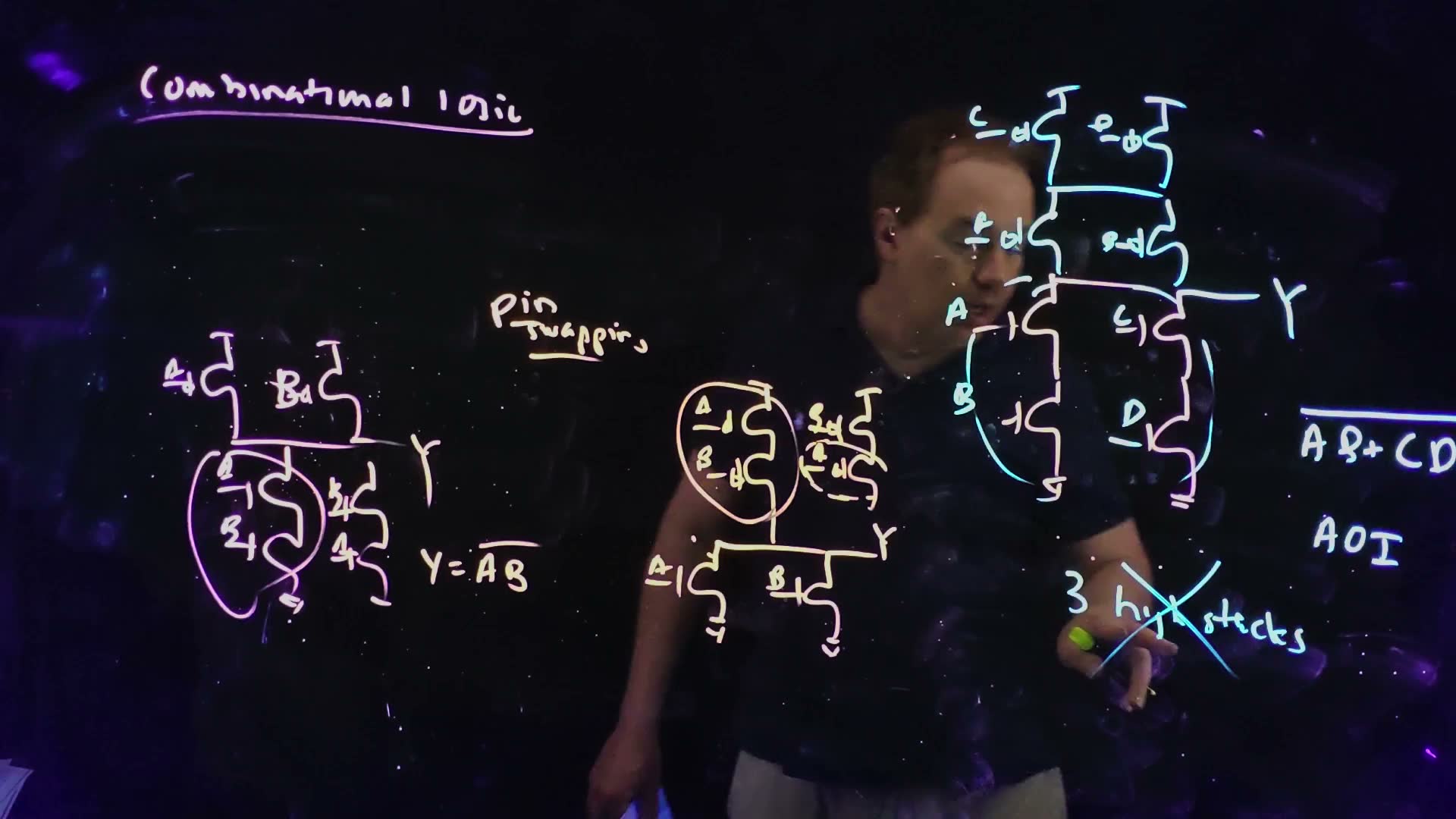
A more complex pull-down (35:49–37:25) board: A and B in series, in parallel with C and D in series. The dual pull-up has A and B in parallel, in series with C and D in parallel. The pull-down conducts when $AB + CD$ is true, so

$$Y = \overline{AB + CD},$$

an AND-OR-invert (AOI) gate board. Pin swapping applies here too: the AB and CD branches could change places (36:52). Choose AOI in the widget above to try it.

What limits a gate’s complexity

Why not put a whole block of logic into one huge gate (37:25)? Stacks. In a tall stack, the devices far from the output switch very slowly (37:53) board:

• two high: no problem;
• three high: questionable, but sometimes acceptable;
• more than three high: practically never (38:20).

That is what limits how much logic goes into a single stage of static CMOS.

Check yourself A four-input NAND (all NFETs in one series stack) has one input that arrives much later than the other three. Which stack position should it get, and why?

The position nearest the output. A single input switching near the output gives a shorter delay than one switching at the bottom of the stack (34:15), so the late signal should use the fastest input. (MT17-3d asks how the bottom input compares: it is slower. The reason is in Chapter 8.)

6. A static gate that is not complementary

The idea. If the inputs are guaranteed to come with their complements, some of a dual network’s connections become unnecessary. The gate is still static, though no longer a strict dual.

Lecture07 @ 41:21The constrained gate after the link between the pull-up columns was erased (it is still drawn at 40:31, see the gallery).

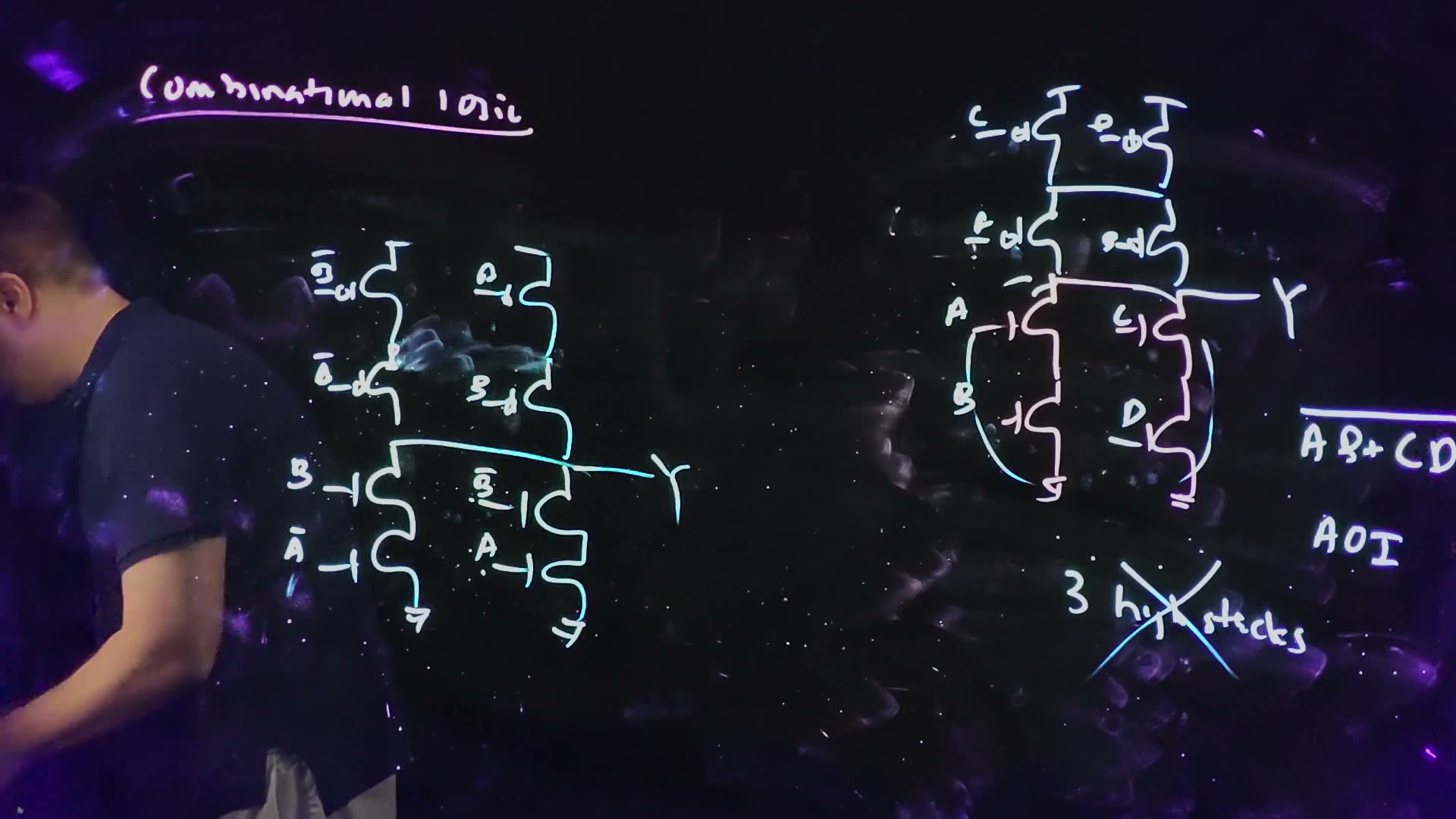
The lecture’s example (38:52–41:15) board:

• the inputs come in complementary pairs: A with Ā, B with B̄, and whatever drives them guarantees that each pair is always opposite (39:31);
• the pull-down: B in series with Ā, in parallel with B̄ in series with A;
• its dual pull-up: B̄ and A in parallel, in series with Ā and B in parallel. Drawn as two columns, B̄ over Ā and A over B, with a link between the middles of the columns (40:08).

The claim (40:20): removing the link changes neither the logic function nor the static behaviour, because the input constraints hold. The result is a static CMOS gate whose networks are not duals (40:44). The lecturer leaves the proof as an exercise.

The proof (added)

1. Pull-down: it conducts when $B\bar A + \bar B A$BˉA, that is, when A and B differ.
2. Pull-up with the link: the PFET pairs conduct when $(B + \bar A)$ and $(A + \bar B)$ are both true. Multiplying out with $\bar A = \text{NOT } A$NOT A: $AB + \bar A\bar B$AˉBˉ, that is, when A and B are equal.
3. Pull-up without the link: the left column (B̄ over Ā) conducts when $B = 1$ and $A = 1$1; the right column (A over B) when $A = 0$ and $B = 0$0. Together: $AB + \bar A\bar B$AˉBˉ, the same.
4. In every one of the four allowed input combinations, exactly one network conducts. The gate is static, and $Y = AB + \bar A\bar B$AˉBˉ: an XNOR (the lecture doesn’t name it).

Choose the two “constrained gate” settings in the widget of Section 4 and compare the truth tables. Then press “Set all four inputs freely” added: with A = 0, Ā = 0, B = 1, B̄ = 1 the gate without the link has neither network on and its output floats, while the full dual still drives it. The link is only unnecessary because of the constraint.

Check yourself In the constrained gate without the link, take A = 1, B = 0 (so Ā = 0, B̄ = 1). Which devices conduct, and what is Y?

Pull-down: the B̄–A branch has both NFETs on (B̄ = 1, A = 1), so it conducts. Pull-up: the left column needs B̄ = 0 (it is 1), the right column needs A = 0 (it is 1); neither conducts. Only the pull-down is on: Y = 0, as an XNOR gives for unequal inputs.

7. The fan-out-of-one delay

The idea. With the delay model, the FO1 delay of an inverter is just $3R_{nfet}C_g$3Rnfet​Cg​, independent of its size. It becomes the unit in which all gate delays are measured: $\tau_{inv}$τinv​.

Lecture07 @ 46:41FO1 = C_g(3W)·R_nfet/W = 3R_nfet C_g = τ_inv (left), and two 2W devices in series acting as one of width W (bottom right).

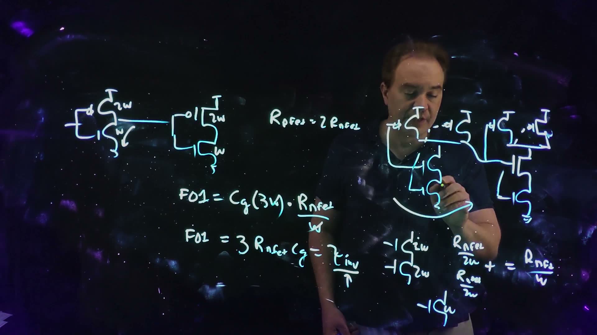
Back to our friend the fan-out of one (41:46): an inverter with a $W$ NFET and a $2W$ PFET drives one identical inverter, with $R_{pfet} = 2R_{nfet}$ so that rise and fall are equal (42:02).

FO1 from the model (board, 42:19–43:26)

1. The load is the next inverter’s input, $W + 2W = 3W$ of gate board: $C_{load} = C_g(3W)$Cg​(3W).
2. Use the pull-down (the pull-up gives the same): resistance $R_{nfet}/W$Rnfet​/W.
3. Multiply board: $\mathrm{FO1} = C_g(3W) \cdot \dfrac{R_{nfet}}{W}$WRnfet​​.
4. The widths cancel board: $\mathrm{FO1} = 3R_{nfet}C_g$3Rnfet​Cg​.

“Once I know my technology parameters, the $C_g$ and $R_{nfet}$Rnfet​, I also can calculate my fan-out of one delay. Isn’t that nice?” (43:11). This delay is called $\tau_{inv}$τinv​, the basic unit of delay (43:26) board.

FO1, the unit of delayboard

$$\tau_{inv} = \mathrm{FO1} = C_g(3W)\,\frac{R_{nfet}}{W}$$$$\tau_{inv} = 3R_{nfet}C_g$$

Independent of $W$W: a bigger inverter is stronger, but its copy is bigger by the same factor.

Holds when: inverter sized 2W/W, R_pfet = 2R_nfet, driving one identical inverter; gate loading only

Compared with Chapter 5. added Lecture 5 found $\mathrm{FO1} = 3\tau_{tr}(1 + 1/\eta)$ and showed that FO4 is less than four times FO1, because the driver’s own drain capacitance is paid only once. This model has no drain capacitance, so here $\mathrm{FO4} = 4\,\mathrm{FO1} = 12R_{nfet}C_g$12Rnfet​Cg​. That is why bench 2’s delay in Section 3 equals $4\tau_{inv}$4τinv​.

Worked example. added With the numbers of Section 3, $R_{nfet} = 2.0\,\mathrm{k\Omega\cdot\mu m}$ and $C_g = 1.00\,\mathrm{fF/\mu m}$1.00fF/μm: $\tau_{inv} = 3 \times 2.0 \times 1.00 = 6\,\mathrm{ps}$6ps, and $\mathrm{FO4} = 24\,\mathrm{ps}$24ps, the delay bench 2 measured. With the lecture’s 2 fF/µm and $R_{nfet} = 2.5\,\mathrm{k\Omega\cdot\mu m}$2.5kΩ⋅μm: $\tau_{inv} = 3 \times 2.5 \times 2 = 15\,\mathrm{ps}$15ps.

Any load in units of τ_inv. added An inverter with NFET $W_n$ (PFET $2W_n$2Wn​) driving $C_{load}$ has delay $\dfrac{R_{nfet}}{W_n}C_{load} = \dfrac{C_{load}}{3W_nC_g}\,\tau_{inv}$3Wn​Cg​Cload​​τinv​: the load divided by the inverter’s own input capacitance, in units of $\tau_{inv}$τinv​. An extra fixed load (a wire, a side branch) just adds to $C_{load}$Cload​.

Common mistakes.

• Counting only the NFET of the receiving inverter. Its input is the gate of both devices, $3W$3W.
• Expecting a bigger inverter to have a smaller FO1. It drives a bigger copy; the widths cancel. Size helps only against a fixed load.
• Assuming every exam uses $R_{pfet} = 2R_{nfet}$2Rnfet​. Some problems state that the NFET and PFET have equal strength; then the balanced inverter is $W/W$ and $\tau_{inv} = 2R_{nfet}C_g$2Rnfet​Cg​. added

Check yourself C_g = 1 fF/µm, R_nfet = 1 kΩ·µm, R_pfet = 2 kΩ·µm. A 2W/W inverter with W = 2 µm drives an identical inverter plus a 4 fF side load. What are τ_inv and the delay?

$\tau_{inv} = 3 \times 1 \times 1 = 3\,\mathrm{ps}$3ps. The load is $3W C_g + 4 = 6 + 4 = 10\,\mathrm{fF}$10fF, the resistance $R_{nfet}/W = 0.5\,\mathrm{k\Omega}$0.5kΩ, so the delay is $0.5 \times 10 = 5\,\mathrm{ps}$5ps. In units of $\tau_{inv}$τinv​: $(6 + 4)/6 = 5/3$5/3, and $5/3 \times 3 = 5\,\mathrm{ps}$5ps. (MT23-1d uses this stage delay.)

Check yourself A chain of four identical 2W/W inverters, each output also carrying a wire of C_x. τ_inv = 20 ps, C_g = 2 fF/µm. What is the delay through the chain for C_x = 0, and for C_x = 6 fF with W = 2 µm and with W = 10 µm? Which W minimizes the delay?

$C_x = 0$0: every stage is an FO1, so $4\tau_{inv} = 80\,\mathrm{ps}$80ps, whatever $W$W. With the wire, each stage is $\tau_{inv}(3WC_g + C_x)/(3WC_g)$Cx​)/(3WCg​). $W = 2\,\mu\mathrm{m}$2μm: $3WC_g = 12\,\mathrm{fF}$12fF, a stage is $20 \times 18/12 = 30\,\mathrm{ps}$30ps, the chain $120\,\mathrm{ps}$120ps. $W = 10\,\mu\mathrm{m}$10μm: $3WC_g = 60\,\mathrm{fF}$60fF, a stage is $20 \times 66/60 = 22\,\mathrm{ps}$22ps, the chain $88\,\mathrm{ps}$88ps. The delay keeps falling as $W$ grows: the wire becomes negligible next to the gates. (MT17-4a–b, MT21-4a, FN10-4a, MT24-2e.)

Check yourself With R_pfet = 2R_nfet and C_g = 2 fF/µm, an inverter with a 2 µm PFET and a 1 µm NFET drives 50 fF. Find both delays in units of τ_inv. Repeat with an 8 µm PFET.

50 fF is 25 µm of gate. Falling: $(R_{nfet}/1\,\mu\mathrm{m}) \times 25\,\mu\mathrm{m}\,C_g = 25R_{nfet}C_g = 25/3 = 8.33\,\tau_{inv}$8.33τinv​. Rising with 2 µm: $(2R_{nfet}/2) \times 25C_g$25Cg​, also $8.33\,\tau_{inv}$8.33τinv​. Rising with 8 µm: $(2R_{nfet}/8) \times 25C_g = 6.25R_{nfet}C_g = 2.08\,\tau_{inv}$2.08τinv​; the falling delay is unchanged. (MT17-3a–b is this problem with equal-strength devices, where $\tau_{inv} = 2R_{nfet}C_g$2Rnfet​Cg​.)

Check yourself An inverter sized W_p/W_n = n µm/1 µm drives an identical inverter (R_pfet = 2R_nfet). Write its falling and rising delays in units of R_nfetC_g. Which gives the smaller sum of the two, n = 2 or n = 1.5?

The load is $(n + 1)$ µm of gate. Falling: $(R_{nfet}/1)(n + 1)C_g = (n + 1)R_{nfet}C_g$1)Rnfet​Cg​. Rising: $(2R_{nfet}/n)(n + 1)C_g$1)Cg​. For $n = 2$2: $3 + 3 = 6$6. For $n = 1.5$1.5: $2.5 + 3.33 = 5.83$5.83, smaller: a narrower PFET loads the previous stage less, and that wins more on the falling edge than it loses on the rising one. (MT21-4c finds the best $n$n, $\sqrt{2}$2​, by calculus; the exam kit does it.)

Check yourself From HW3 you have C_g = 1 fF/µm, R_nfet = 3 kΩ·µm and R_pfet = 6 kΩ·µm. An inverter with an 8 µm PFET and a 4 µm NFET drives an identical inverter. Estimate t_pLH and t_pHL.

The load is $(8 + 4) \times 1 = 12\,\mathrm{fF}$12fF. $t_{pLH} = (6/8) \times 12 = 9\,\mathrm{ps}$ and $t_{pHL} = (3/4) \times 12 = 9\,\mathrm{ps}$9ps. (HW4-1b does this with its own characterized values.)

8. Sizing stacks and logical effort

The idea. To give a NAND or NOR the same drive as an inverter, the stacked devices must be made wider. Wider devices mean more input capacitance for the same drive, so the gate is slower than an inverter by a fixed factor: its logical effort.

Two devices in series

Treat stacked transistors like resistors in series (45:29) board:

The stack rule (board, 45:29–46:28)

1. Two NFETs in series, each of width $2W$2W. Each has resistance $R_{nfet}/2W$Rnfet​/2W.
2. In series the resistances add board: $\dfrac{R_{nfet}}{2W} + \dfrac{R_{nfet}}{2W} = \dfrac{R_{nfet}}{W}$WRnfet​​.
3. That is the resistance of a single NFET of width $W$ board.
4. So a stack of two needs each device twice as wide to keep the strength of one device. (“Zero order”, the lecturer adds (46:00).)

added The same counting for a stack of three: each device $3W$3W, since $3 \times R/3W = R/W$R/W.

NAND driving NAND

Lecture07 @ 50:42NAND driving NAND, every device 2 µm, against the 2/1 µm inverter: delay = C_g(4 µm) R_nfet/1 µm = 4/3 τ_inv, the logical effort.

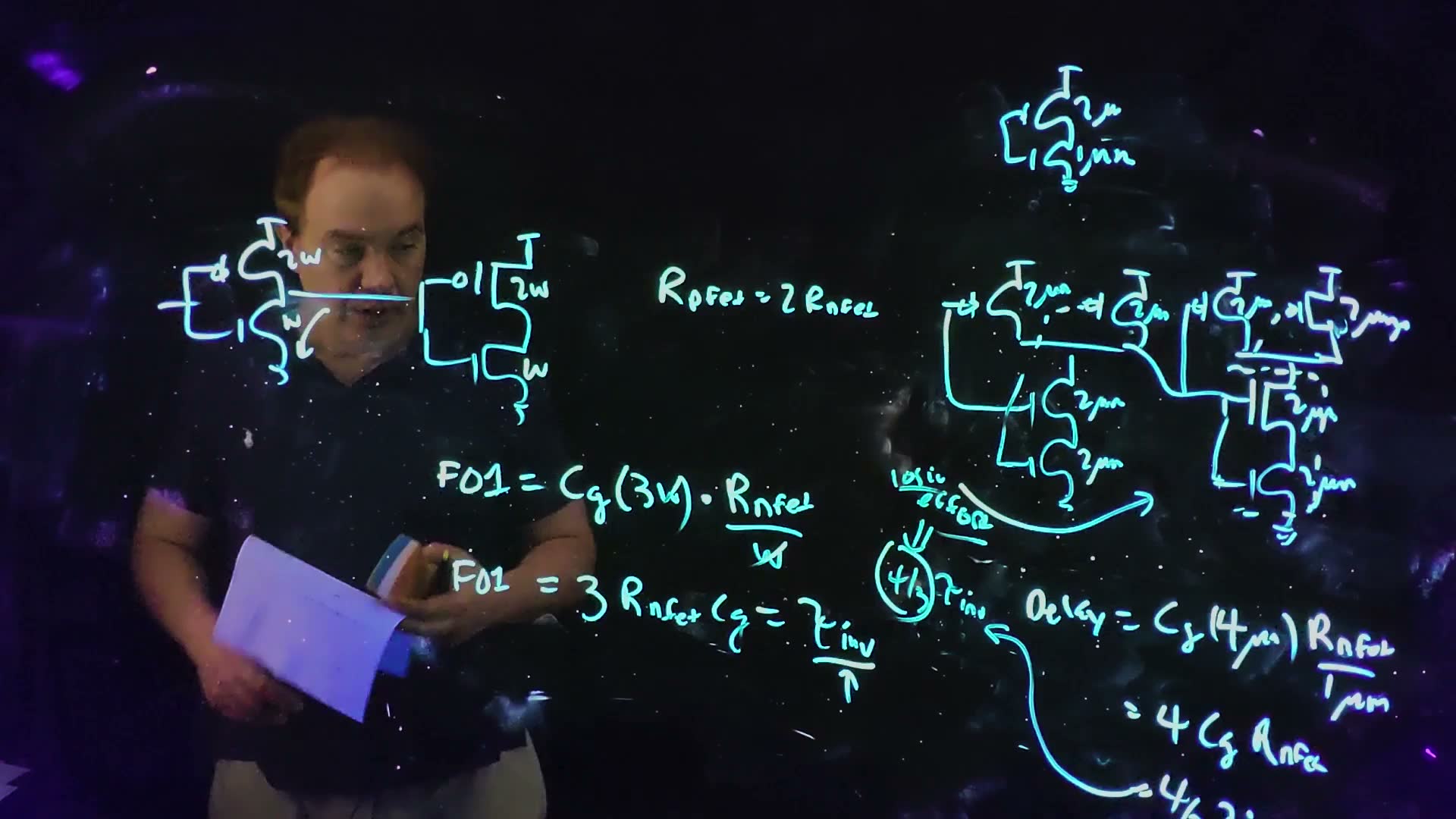
Size a NAND to match a 2/1 µm inverter (46:28–47:12) board:

• its two NFETs are in series, so each is 2 µm: together they act like the inverter’s 1 µm NFET;
• its two PFETs are in parallel, each 2 µm, like the inverter’s 2 µm PFET. added Why not 1 µm each, since two in parallel make 2 µm? Because when only one input falls, only one PFET turns on, and it alone must match the inverter’s pull-up. Sizing is for the worst case.

Now let the NAND drive an identical NAND (47:25):

NAND logical effort (board, 47:47–50:31)

1. One input of the receiving NAND is the gate of one 2 µm NFET and one 2 µm PFET: $4\,\mu\mathrm{m}$ of gate board.
2. The driving NAND pulls down with the strength of a 1 µm NFET, $R_{nfet}/1\,\mu\mathrm{m}$Rnfet​/1μm.
3. Delay board: $C_g(4\,\mu\mathrm{m}) \cdot \dfrac{R_{nfet}}{1\,\mu\mathrm{m}} = 4C_gR_{nfet}$4Cg​Rnfet​.
4. Since $C_gR_{nfet} = \tau_{inv}/3$ board: delay $= \tfrac43\,\tau_{inv}$34​τinv​.

Why 4/3 (49:16). The NAND has the same drive strength as the 2/1 inverter, but it presents 4 µm of input capacitance instead of 3 µm. Building the more complex function needed a stack, the stack needed larger devices, and larger devices are more capacitance to drive. (At 49:03 the lecturer says “four thirds the drive strength”; he means four thirds the delay, as he said a sentence earlier and as the board writes.)

This number, $4/3$4/3, is the logical effort of the NAND (49:47) board. It is a property of the gate’s structure: with every device $W$ instead of 2 µm, the same calculation gives $4/3\,\tau_{inv}$ again (50:03).

NOR driving NOR

Lecture07 @ 53:53NOR driving NOR: PFETs 4W, NFETs W; delay = C_g 5W R_nfet/W = 5/3 τ_inv.

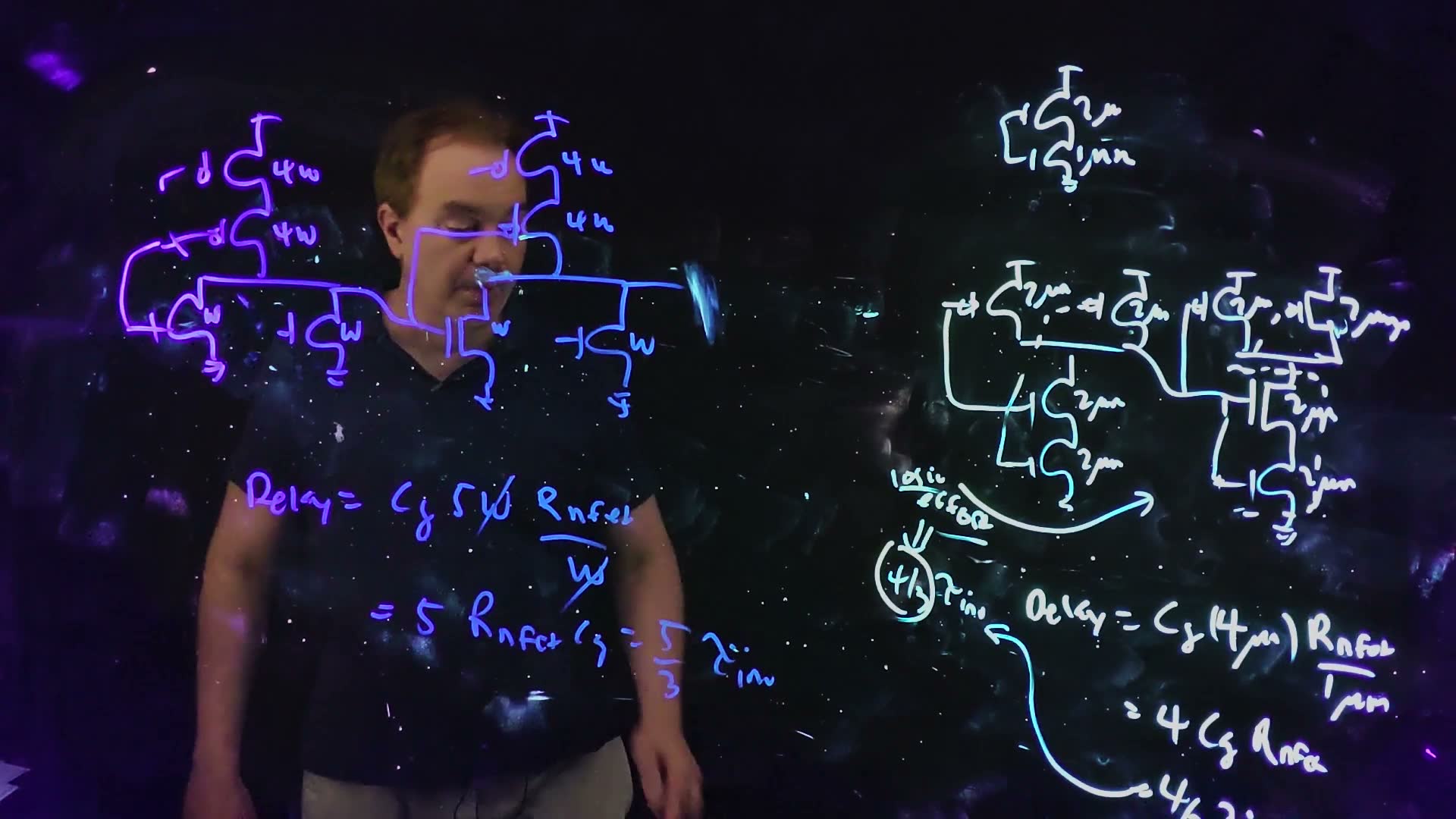
Will the NOR’s logical effort be better or worse (50:35)? Worse: the NOR stacks the PFETs, which are already twice as large, and stacking doubles them again (51:06).

NOR logical effort (board, 52:43–53:52)

1. NFETs in parallel, each $W$W: one alone has the strength of the inverter’s $W$ NFET.
2. A single PFET would need $2W$2W; two in series need twice that: $4W$ each board.
3. One input: $W + 4W = 5W$ of gate.
4. Delay board: $C_g(5W) \cdot \dfrac{R_{nfet}}{W} = 5R_{nfet}C_g = \tfrac53\,\tau_{inv}$35​τinv​.

The logical effort is 5/3, worse than the NAND’s 4/3, “just as we suspected” (53:52).

Sizing stacks and logical effortboard

$$\text{stack of } n:\ \text{each device } n \times \text{wider}$$$$g = \frac{C_{in,\,gate}}{C_{in,\,inverter}} = \frac{\text{delay driving a copy}}{\tau_{inv}}$$$$g_{inv} = 1, \quad g_{NAND2} = \tfrac43, \quad g_{NOR2} = \tfrac53$$

NAND: NFETs $2W$2W, PFETs $2W$2W, $C_{in} = 4W\,C_g$4WCg​. NOR: NFETs $W$W, PFETs $4W$4W, $C_{in} = 5W\,C_g$5WCg​. Both have the inverter’s drive.

Holds when: each gate sized for the drive of a 2W/W inverter, R_pfet = 2R_nfet; driving one identical gate; gate loading only. The general definition g = C_in/(3W C_g) is added

Compare the gates, and see what the fan-out and an extra load do:

inverterNAND2NOR2NAND3NOR3

fan-out: copies of the same gate driven

1

extra load C_x (wire, side branch)

0 fF

reference NFET width W

1.0 µm

R_nfet (R_pfet = 2R_nfet)

2.0 kΩ·µm

C_g

1.0 fF/µm

NFETs

2 in series, 2 µm each

PFETs

2 µm each, 2 in parallel

one input's gate width

4 µm = 4.00 fF

logical effort g = C_in/(3W C_g)

1.333

electrical effort h = C_out/C_in

1.000

gain g·h

1.333

τ_inv = 3R_nfetC_g

6.00 ps

delay (R_nfet/W) × C_out

8.00 ps = 1.333 τ_inv

Each line's slope is its logical effort: every extra copy driven adds one more C_in, and the gate's drive is the same as the reference inverter's. With C_x = 0 the widths cancel: change W, R_nfet or C_g and the delay in τ_inv stays put. A fixed extra load breaks that: larger W makes it relatively smaller. Drain capacitance is ignored, as in the lecture's model. The lecture works the inverter, NAND2 and NOR2; the 3-input gates use the same stack rule.

What to notice.

• With fan-out 1 the delays are $1$1, $4/3$ and $5/3\,\tau_{inv}$5/3τinv​, whatever $W$W, $R_{nfet}$ or $C_g$Cg​: logical effort is a pure number.
• Each line’s slope is its logical effort. NOR2 and NAND3 lie on top of each other: both have $g = 5/3$5/3.
• Add an extra load $C_x$ and the delay depends on $W$ again; a larger $W$ helps (Section 7’s chain).

Worked example. added With $\tau_{inv} = 6\,\mathrm{ps}$ (Section 3’s technology): a NAND driving a NAND takes $\tfrac43 \times 6 = 8\,\mathrm{ps}$8ps, a NOR driving a NOR $\tfrac53 \times 6 = 10\,\mathrm{ps}$10ps. The NAND is the faster of the two.

Common mistakes.

• Counting all four transistors of the receiving gate. One input connects to one NFET and one PFET; only those are its load.
• Sizing the parallel devices as if they all turn on together. A single one may be the only one on.
• Forgetting that the PFET doubling and the stack doubling multiply in the NOR: $2 \times 2W = 4W$4W.

Check yourself Size the AOI gate of Section 5 for the drive of a 2W/W inverter, and find its logical effort for input A.

Pull-down: each branch is a stack of two NFETs, so each is $2W$2W. Pull-up: two parallel pairs in series, a stack of two PFETs in the worst case, so each PFET is $2 \times 2W = 4W$4W. Input A drives one $2W$ NFET and one $4W$ PFET: $6W$ of gate. $g = 6W/3W = 2$2.

Check yourself A four-input NAND has all four NFETs and all four PFETs 4 µm wide; it drives 50 fF, with C_g = 2 fF/µm and R_pfet = 2R_nfet. Find the falling and rising delays in units of τ_inv.

50 fF is 25 µm of gate. Falling: four 4 µm NFETs in series act as one 1 µm NFET, so $(R_{nfet}/1) \times 25C_g = 25R_{nfet}C_g = 8.33\,\tau_{inv}$8.33τinv​. Rising: one 4 µm PFET, $(2R_{nfet}/4) \times 25C_g = 12.5R_{nfet}C_g = 4.17\,\tau_{inv}$4.17τinv​. (MT17-3d, with equal-strength devices in the original.)

9. Electrical effort and gain

The idea. A gate’s delay is the product of two factors: its logical effort $g$ (how much harder its structure is to drive than an inverter’s) and its electrical effort $h$ (how much load it drives compared with its own input). The product $g \cdot h$ is the gate’s gain, and the delay is gain × $\tau_{inv}$τinv​.

Lecture07 @ 57:19A NAND driving two NANDs: (2)(4/3) τ_inv. h = 2 is the electrical effort, g = 4/3 the logical effort, their product the gain.

Let the NAND drive two NANDs of its own size (54:35):

Gain (board, 54:57–56:20)

1. The load doubles: two inputs of 4 µm each board: $C_g(4\,\mu\mathrm{m})(2)$Cg​(4μm)(2).
2. Delay board: $C_g(4\,\mu\mathrm{m})(2)\,\dfrac{R_{nfet}}{1\,\mu\mathrm{m}} = 2 \times \tfrac43\,\tau_{inv} = \tfrac83\,\tau_{inv}$38​τinv​.
3. The $\tfrac43$ is the logical effort, $g$ board.
4. The extra factor 2, from fanning out to two gates of the same size, is the electrical effort, $h$ board. In the Sutherland and Sproull book they are called $g$ and $h$ (55:53).
5. Their product is the gain of the gate board: $g \cdot h = \tfrac83$38​.

The gain is “the factor that I multiply by $\tau_{inv}$τinv​, the unit inverter delay, to get the delay of that gate given its loading” (56:20).

Gainboard

$$\text{delay} = g \cdot h \cdot \tau_{inv}, \qquad h = \frac{C_{out}}{C_{in}}$$

Holds when: gate loading only; g from Section 8; h is the load divided by the gate's own input capacitance (driving N copies of itself gives h = N; the general ratio is added)

What comes next (56:31). The next lecture uses gains to estimate the delay of any path through logic “very quickly and easily”, and then to choose the transistor widths along a critical path that minimize its delay: gain-based tuning, also called the method of logical effort, after the Sutherland and Sproull book on the course reserves (57:04). added Since each gate’s delay is its own gain times $\tau_{inv}$τinv​, a path’s delay is the sum of the gains along it, times $\tau_{inv}$τinv​.

Worked example. added With $\tau_{inv} = 6\,\mathrm{ps}$6ps: the NAND driving two NANDs takes $\tfrac83 \times 6 = 16\,\mathrm{ps}$16ps. Set the widget of Section 8 to NAND2 with fan-out 2 to see it.

Check yourself An inverter (2 µm PFET, 1 µm NFET) drives one input of a NAND sized like the lecture's (every device 2 µm). The NAND drives 60 fF. With C_g = 2 fF/µm and R_pfet = 2R_nfet, what is each stage's gain, and the total delay in τ_inv?

Inverter: $g = 1$1, $h = 4\,\mu\mathrm{m}/3\,\mu\mathrm{m} = 4/3$4/3, gain $1.33$1.33. NAND: $g = 4/3$4/3; 60 fF is 30 µm of gate, so $h = 30/4 = 7.5$ and the gain is $10$10. Total: $1.33 + 10 = 11.33\,\tau_{inv}$11.33τinv​. Check the NAND directly: $(R_{nfet}/1\,\mu\mathrm{m}) \times 60\,\mathrm{fF} = 30R_{nfet}C_g = 10\,\tau_{inv}$10τinv​. (MT17-5a and MT23-5a add gains this way along four stages.)

Check yourself A NOR (logical effort 5/3) drives three NORs of its own size. What is its gain? With τ_inv = 15 ps, what is its delay?

$h = 3$3, so the gain is $\tfrac53 \times 3 = 5$5, and the delay $5 \times 15 = 75\,\mathrm{ps}$75ps.

Formulas to remember

Formula	Meaning
$t = \dfrac{R}{W}\,C_{load}$WR​Cload​; $1\,\mathrm{k\Omega} \times 1\,\mathrm{fF} = 1\,\mathrm{ps}$	the simplified delay model; $R$ is a fitted constant (no ln 2)
$C_g/W = L\kappa_{ox}\varepsilon_0/t_{ox} \approx 2\,\mathrm{fF/\mu m}$	gate capacitance per micron; constant under scaling
$R_{nfet}$Rnfet​, $R_{pfet}$ in kΩ·µm, $R_{pfet} \approx 2R_{nfet}$	resistance times width; divide by $W$
$C_g = C_L/(8(16 + 8)\,\mu\mathrm{m})$	bench 1: match $C_L$ to an 8(16/8) input
$R_{nfet} = \dfrac{t_{pHL}}{C_L}4(8\,\mu\mathrm{m})$CL​tpHL​​4(8μm), $R_{pfet} = \dfrac{t_{pLH}}{C_L}4(16\,\mu\mathrm{m})$	bench 2, $C_L = C_g \cdot 16(16 + 8)\,\mu\mathrm{m}$8)μm; AS = AD = PS = PD = 0
exactly one of PUN, PDN on	static CMOS (both on: ratioed; both off: dynamic)
PUN and PDN duals: series ↔ parallel	complementary static CMOS
$\overline{A + B}$A+B​, $\overline{AB}$AB, $\overline{AB + CD}$	NOR, NAND, AOI
late signal on the device nearest the output; stacks ≤ 2, maybe 3	pin swapping; the stack limit
$\tau_{inv} = \mathrm{FO1} = 3R_{nfet}C_g$	the unit of delay; FO4 = $4\tau_{inv}$ in this model
stack of $n$n: each device $n\times$ wider	equal drive
$g_{NAND2} = 4/3$4/3, $g_{NOR2} = 5/3$	logical effort, $C_{in,gate}/C_{in,inv}$
delay $= g \cdot h \cdot \tau_{inv}$τinv​, $h = C_{out}/C_{in}$	gain

The lecture’s boards

Lecture07 @ 04:21 trajectories; the switch-and-resistor model

Lecture07 @ 09:32 C_g in fF/µm; R_nfet, R_pfet in kΩ·µm

Lecture07 @ 18:15 bench 1: C_g = C_L/(8(16+8) µm)

Lecture07 @ 24:54 bench 2: R_nfet, R_pfet; AS = AD = PS = PD = 0

Lecture07 @ 31:52 static CMOS; duals; the NOR

Lecture07 @ 34:56 NAND; pin swapping

Lecture07 @ 38:24 AOI; no tall stacks

Lecture07 @ 40:31 constrained gate, link drawn

Lecture07 @ 41:21 constrained gate, link removed

Lecture07 @ 46:41 FO1 = 3R_nfet C_g = τ_inv; stack rule

Lecture07 @ 50:42 NAND logical effort 4/3

Lecture07 @ 53:53 NOR logical effort 5/3

Lecture07 @ 57:19 electrical effort, gain