H2. Homework 2: device parameters from simulated I–V curves

Homework 2 is one problem in three parts, all about reading a transistor’s parameters off simulated curves. A 60 nm NFET was simulated in Cadence: a family of $I_D$–$V_{DS}$ curves for (a), a $V_{GS}$ sweep at small $V_{DS}$ for (b), and the same family for a channel 3.3 times longer for (c). From the curves you estimate the saturation velocity, the threshold and the subthreshold slope, and explain why the longer device gives a different number.

There is no simulator in this guide, so this page does not produce new readings. It takes the readings from the key’s plots, redoes the key’s arithmetic from them, and checks the key’s explanations against Chapter 4. Most of the page is about the skill underneath: reading an I–V family, and telling velocity saturation from the square law. That is what the midterm’s short answers need.

After this page you can:

1. read an $I_D$–$V_{DS}$ family and say whether the device is velocity-saturated or follows the square law, from three signs: the spacing between curves, where they flatten, and how the current scales with $L$L;
2. turn two curves’ currents into $v_{sat}$ with $C_{ox}$ from $t_{ox}$tox​, and say why $V_T$ drops out;
3. extract $V_T$ from a low-$V_{DS}$ sweep by linear extrapolation, with the $V_{DS}/2$ correction;
4. read a subthreshold slope in mV/decade from two points of a log plot, and say which way is better;
5. explain why the same method gives a lower number for a longer channel, although $v_{sat}$ hasn’t changed.

Before you start

The source is the key alone. The homework’s question text is not in the source, only the key (homework2_solution, 3 pages). Each part below is restated from what the key’s text says it does, so read the restatements as “the task the key solves”, not as the original wording.

How to use this page. Section 2 is the approach for all three parts: how to read an I–V family, and the three signs that tell velocity saturation from the square law. Read it first. Then every part is worked the same way: what it asks, the idea behind the method, the solution in steps (each step gives its reason first), a check on the result, the answer, and one thing to remember. Try each part on your own first; open the Hint if you are stuck. The key’s verdict is the folded note on the key at the end of each part, and the table at the end lists the disagreements.

Part	Points	Key’s page	What it asks	Chapter 4 sections
HW2-1a	35	p1	$v_{sat}$ from the $I_D$–$V_{DS}$ family, $L = 60$ nm	§5, §7
HW2-1b	30	p1–2, notes p3	$V_T$VT​, and the subthreshold slope	§8, §11
HW2-1c	35	p2, notes p3	$v_{sat}$ again for $L = 200$ nm, and why it differs	§1, §7

Two kinds of reading. Every number on this page comes from the key’s screenshots, in one of two ways:

• Printed markers. Cadence prints a marker’s coordinates on the plot (for example “1.0 460.105uA”). These are quoted exactly as printed.
• Read by eye. The other curves have no markers. Their values here were read from the figures (pixel positions checked against the axis labels and the printed markers) and are good to about ±3 µA. They are marked ≈.

Units. Device work uses centimetres (Chapter 0). With $t_{ox}$ in cm, $C_{ox}$ comes out in F/cm²; the key works in F/m² and gets the same velocities.

1. The benches: what was simulated

HW2, p1: the bench for part (a) (crop of the key’s screenshot). W = 500 nm, L = 60 nm.

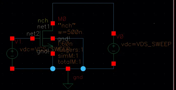
One NFET, source and body grounded, with a voltage source on the gate and one on the drain. With the source grounded, the two sources set $V_{GS}$ and $V_{DS}$ directly; with the body grounded too, $V_{SB} = 0$0, so the body effect plays no part. Three sweeps, each chosen to expose one parameter:

1. Part (a): the output family. $V_{DS}$ swept from 0 to 1.0 V for ten gate voltages, $V_{GS} = 0.1, 0.2, \dots, 1.0$ V. Device $W = 500$ nm, $L = 60$ nm; the key gives $t_{ox} = 2.1$ nm. The gate steps are equal, so the spacing between neighbouring curves shows how the saturated current grows with the overdrive: the one thing that tells the two models apart (Section 2).
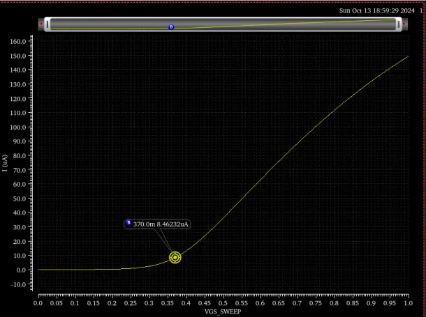
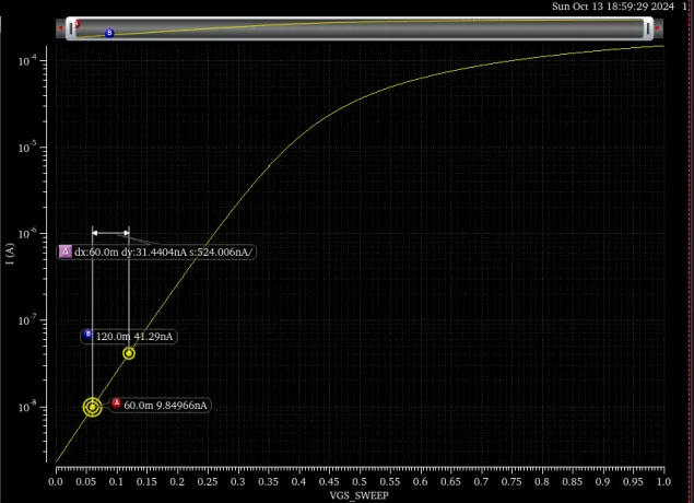
2. Part (b): the transfer sweep. $V_{DS}$ held at 100 mV (the schematic’s vdc=100.0m), $V_{GS}$ swept from 0 to 1.0 V. A drain voltage this small keeps the device in triode at every gate voltage well above threshold, where the current is a straight line in $V_{GS}$VGS​; that line is what the threshold is extracted from. The same curve is plotted twice: on a linear axis for $V_T$VT​, and on a log axis for the subthreshold slope, because below threshold the current is exponential and only a log axis shows it as a line.
3. Part (c): the output family again, with $L = 200$ nm (l=200n), 3.3 times longer. Everything else is the same, so any difference from part (a) comes from the length alone.

These are the measurements of Chapter 4, Section 8 and Section 11, done on a simulated device instead of a real one. The benches of Homework 3, which turn a simulated delay or energy into a resistance, a capacitance or a crowbar share, are taught on H3’s simulation-bench section; the habit is the same: say what the bench holds fixed, what it sweeps, and which formula turns the reading into the parameter.

2. Reading an I–V family: velocity saturation or the square law?

HW2-1a, p1: the key’s I_D–V_DS family for L = 60 nm, V_GS = 0.1 to 1.0 V. Markers A and B are at V_DS = 1.0 V on the top two curves.

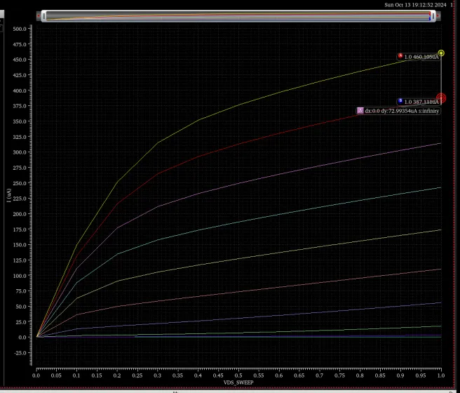
Before computing anything, look at the family: the right formula for every part depends on which model the device follows, and the curves say so before any arithmetic. Chapter 4 gives two models for the saturated current, and they leave different fingerprints. Both start from current = width × channel charge per area × carrier velocity, with the charge $C_{ox}(V_{GS} - V_T)$ (Chapter 4, Section 5); they differ in the velocity.

• Square law (Chapter 4, Section 4): $I_{DSAT} = \dfrac{\mu C_{ox}}{2}\dfrac{W}{L}(V_{GS} - V_T)^2$VT​)2. It holds in a long channel, where the velocity is the mobility $\mu$ times a field that grows with the overdrive, so the overdrive enters twice.
• Fully velocity-saturated (Chapter 4, Section 7): $I_{DSAT} = C_{ox}Wv_{sat}(V_{GS} - V_T)$VT​). It holds when $(V_{GS} - V_T)/L \gg \mathcal{E}_{crit}/2$Ecrit​/2, where $\mathcal{E}_{crit} = v_{sat}/\mu$vsat​/μ: the field is so high that the carriers move at the ceiling $v_{sat}$ whatever the overdrive, so the overdrive enters once.

Real short devices sit between the two, with Chapter 4’s full formula $I_{DSAT} = C_{ox}Wv_{sat}(V_{GS} - V_T)\frac{s - 1}{s + 1}$VT​)s+1s−1​, $s = \sqrt{1 + 2\mu(V_{GS} - V_T)/(v_{sat}L)}$1+2μ(VGS​−VT​)/(vsat​L)​: the factor $\frac{s - 1}{s + 1}$ approaches 1 as the channel shortens, and the formula becomes the square law as it lengthens (Chapter 4’s “other limit” added). The three signs below tell you how far toward either end a family is.

Sign 1: the spacing between the curves

Read every curve at the same $V_{DS}$VDS​, well into saturation (the right edge, 1.0 V), and take the differences between neighbours. Saturation, because both models describe the saturated current; the same $V_{DS}$VDS​, because the curves still slope up there (Sign 2), and at one $V_{DS}$ that slope adds about the same to each curve.

• Velocity-saturated: the current is linear in $V_{GS}$VGS​, so each 0.1 V step of $V_{GS}$ adds the same current, $C_{ox}Wv_{sat}\times 0.1\,\mathrm{V}$0.1V. Equal spacing.
• Square law: $(V_{GS} - V_T)^2$ grows faster and faster, so the steps grow in proportion to the overdrive. Starting from $V_T$VT​, equal $V_{GS}$ steps give currents in the ratio 1 : 4 : 9 : 16, so steps in the ratio 1 : 3 : 5 : 7.

Here are the key’s two families at $V_{DS} = 1.0$ V. Bold values are the printed markers; ≈ values are read by eye.

VGS (V)	ID, L = 60 nm (µA)	step	ID, L = 200 nm (µA)	step
0.3	≈ 15	≈ 14	≈ 2.5	≈ 2
0.4	≈ 54	≈ 39	≈ 12	≈ 9.5
0.5	≈ 108	≈ 54	≈ 29.5	≈ 17.5
0.6	≈ 172	≈ 64	≈ 56	≈ 26.5
0.7	≈ 241	≈ 69	≈ 88.5	≈ 32.5
0.8	≈ 313	≈ 72	≈ 124.5	≈ 36
0.9	387.111	≈ 74	162.71	≈ 38
1.0	460.105	72.99	201.115	38.40

What the table says.

• For $L = 60$ nm the top four steps are 69 to 74 µA: nearly equal. Over the upper half of the range the current is linear in $V_{GS}$VGS​, the velocity-saturated fingerprint. The key says the same in its first sentence.
• Near threshold the steps still grow (14, 39, 54 µA). That is expected even in a short device: the criterion for full saturation is $(V_{GS} - V_T)/L \gg \mathcal{E}_{crit}/2$ (Chapter 4, Section 7), and at small overdrive the field is small. Just above threshold every device looks more like the square law.
• For $L = 200$ nm the steps level off later and less: 26.5, 32.5, 36, 38 µA. The top steps are close, but the levelling starts higher up. That device is less velocity-saturated, because at the same overdrive its field $(V_{GS} - V_T)/L$ is 3.3 times smaller, so it needs a larger overdrive before the field outgrows $\mathcal{E}_{crit}/2$Ecrit​/2.
• Neither family is square-law at the top. A square law would make the 0.9–1.0 V step about 20% larger than the 0.8–0.9 V step: its steps grow in proportion to the overdrive at their midpoints, 0.60 V against 0.50 V with $V_T \approx 0.35$ V. In both families the two top steps agree to within the reading error.

Sign 2: where the curves flatten

In the square law a curve flattens at $V_{DSAT} = V_{GS} - V_T$VT​, where the channel pinches off at the drain: about 0.6–0.65 V for the top curve here. With velocity saturation it flattens earlier and lower (Chapter 4, Section 7), because the carriers reach $v_{sat}$ before the channel pinches off: $V_{DSAT} = 2(V_{GS} - V_T)/(1 + s)$s), less than $V_{GS} - V_T$ whenever $s > 1$1. In the 60 nm family the top curve bends over between about 0.2 and 0.4 V. In the 200 nm family it bends a little later, around 0.4–0.5 V, because its $s$ is smaller (the length sits under the root), which brings $V_{DSAT}$ closer to $V_{GS} - V_T$VT​. Both bend well before $V_{GS} - V_T$VT​, the shorter one sooner.

The curves keep rising past the bend. They don’t go flat as both of Chapter 4’s models say. That upward slope is the finite output conductance of a short device, mostly DIBL (Chapter 4, Section 12): a higher $V_{DS}$ widens the drain’s depletion region under the gate, so the gate supports less depletion charge, $V_T$ falls, and the overdrive and the current grow. It is why you read every curve at the same $V_{DS}$VDS​: then the slope adds about the same error to each curve and mostly cancels in the differences.

Sign 3: how the current scales with L

Compare the two devices at the same bias. The printed markers at $V_{GS} = V_{DS} = 1.0$ V give

$$\frac{I_D(60\,\mathrm{nm})}{I_D(200\,\mathrm{nm})} = \frac{460.105}{201.115} = 2.29 .$$

• Square law: $I \propto 1/L$1/L, because the same voltage across a longer channel is a weaker field and a slower drift, so the ratio would be $200/60 = 3.33$3.33.
• Fully velocity-saturated: $I$ doesn’t depend on $L$ at all (Chapter 4, Section 7), because charge × $v_{sat}$ contains no length: the carriers move at the ceiling in either device. The ratio would be 1.

The answer, 2.29, lies between the two: neither device is fully velocity-saturated, and the shorter one is closer. The steps tell the same story added: $72.99/38.40 = 1.90$1.90, also between 1 and 3.33. This sign is the strongest of the three, because it uses only printed markers; the first two lean on readings by eye.

Try it

The widget uses Chapter 4’s velocity-saturated model with this homework’s geometry ($W = 0.5$W= µm, $t_{ox} = 2.1$ nm, $V_{DD} = 1$ V) and the chapter’s illustrative $\mu$ and $v_{sat}$vsat​. The bottom plot divides each step by the top step. The coloured dots are the key’s two families from the table above (read by eye, so the lower dots are rough).

L:60 nm200 nm1000 nm

channel length L

60.0 nm

threshold V_T

0.35 V

(V_DD − V_T)/L vs ℰ_crit/2

108 vs 12.5 kV/cm (×8.67)

top step, velocity-saturated model

54.8 µA

top step if the square law held

329 µA

step method: ΔI/(C_oxWΔV)

6.66×10⁶ cm/s

as a share of the model's v_sat

67%

Top: the saturated current at each V_GS of Chapter 4's velocity-saturated model (blue; dots at the 0.1 V steps), the square law for the same device (orange, dashed; cut off once it passes the top of the grey line, which it does for short channels) and the full-saturation limit C_oxWv_sat(V_GS − V_T) (grey, dotted). Bottom: each step between neighbouring V_GS curves divided by the top step; coloured dots, if shown, are readings passed in by the page. Equal steps (a flat line at 1) mean velocity saturation; steps that grow in proportion to the overdrive (a line through V_T) mean the square law. Device: W = 0.5 µm, t_ox = 2.1 nm, μ = 400 cm²/V·s, v_sat = 10⁷ cm/s (Chapter 4's illustrative values), ℰ_crit = 25 kV/cm. This is the course model, not the simulator.

What to notice.

• Equal steps are a flat line at 1; the square law is a straight line through $V_T$VT​. Each step is divided by the top step, so equal steps all come out at 1; square-law steps grow in proportion to the overdrive at their midpoints, so they fall on a line that reaches zero at $V_T$VT​. The 60 nm dots run flat at the top; the 200 nm dots bend toward the square-law line sooner.
• Press 200 nm, then 1000 nm: the model’s step curve moves from the flat line toward the square-law line, and the share of $v_{sat}$ that the step method recovers falls (67% at 60 nm, 46% at 200 nm, with $V_T = 0.35$ V), because a longer channel has a smaller $s$ and so a smaller factor $\frac{s - 1}{s + 1}$s+1s−1​. Part (c) is this effect.
• The model is not the simulator. Its currents are smaller than the key’s, and its dots don’t sit on the key’s dots. Only the direction of the trend carries over.

Check yourself Two NFETs are measured at the same V_DS = V_DD, at V_GS = 0.6, 0.8 and 1.0 V. Device X gives 100, 200 and 300 µA; device Y gives 20, 80 and 180 µA. Which follows the square law, which is velocity-saturated, and roughly where is Y's threshold?

X: steps of 100 and 100 µA, equal, so the current is linear in $V_{GS}$VGS​: velocity-saturated. Y: steps of 60 and 100 µA, growing. Test the square law: $\sqrt{20} : \sqrt{80} : \sqrt{180} = 1 : 2 : 3$3, so $V_{GS} - V_T$ is in the ratio 1 : 2 : 3 at 0.6, 0.8 and 1.0 V. That puts $V_T$ at 0.4 V (overdrives 0.2, 0.4, 0.6 V). Y follows the square law with $V_T = 0.4$ V.

Check yourself A short-answer question: why does a short-channel MOSFET's saturation current grow only linearly with V_GS − V_T, when the long-channel current grows as its square?

$I_D = W\,Q_i\,v$WQi​v. The overdrive enters the long-channel current twice: in the charge $Q_i = C_{ox}(V_{GS} - V_T)$ and in the drift velocity, through the field. In a short channel the field is so high that the carriers move at $v_{sat}$vsat​, whatever the overdrive, so only the charge factor is left: $I_{DSAT} = C_{ox}Wv_{sat}(V_{GS} - V_T)$ (Chapter 4, Section 5).

3. HW2-1a: the saturation velocity from two curves

HW2-1a, p1 (35 points), restated from the key. The family above shows $I_D$ against $V_{DS}$ for $V_{GS}$ from 0.1 V to 1.0 V in steps of 0.1 V, for an NFET with $W = 500$ nm and $L = 60$ nm. With $t_{ox} = 2.1$ nm, estimate the saturation velocity $v_{sat}$vsat​.

Hint

At the top of the family the curves are evenly spaced. Which of Chapter 4’s two models gives equal steps, and what is left of its formula when you subtract two curves?

What it asks. The saturation velocity $v_{sat}$vsat​, the ceiling on the electrons’ drift velocity, from the family of output curves in Section 2. You know the device’s geometry and $t_{ox}$tox​, but not its threshold: part (b) finds that later. “Saturation velocity”, with a family of equal gate steps to read from, decides the method: the step between two curves.

The idea. Section 2’s first sign found the top curves evenly spaced, the velocity-saturated fingerprint. In that limit the saturated current is Chapter 4’s

$$I_D = C_{ox}Wv_{sat}(V_{GS} - V_T)$$

the channel charge per area $C_{ox}(V_{GS} - V_T)$VT​), times the width, times the ceiling velocity. It holds when $(V_{GS} - V_T)/L \gg \mathcal{E}_{crit}/2$ (Chapter 4, Section 7). Subtract two curves read at the same $V_{DS}$VDS​:

$$\Delta I_D = C_{ox}Wv_{sat}\,\Delta V_{GS}$$ $$v_{sat} = \frac{\Delta I_D}{C_{ox}W\,\Delta V_{GS}}$$

$V_T$ cancels in the difference, so you don’t need part (b) first. The tempting shortcut, dividing one current by $C_{ox}W(V_{GS} - V_T)$VT​), needs $V_T$VT​, and it also counts the upward slope past the bend (Sign 2), which the difference cancels.

The step method, from the readings on the key's plot

1. Pick the two curves. The formula assumes full velocity saturation, and the top steps are the flattest (Section 2), so use the top two curves, $V_{GS} = 1.0$ and 0.9 V. Read both at $V_{DS} = 1.0$ V, so that the upward slope cancels.
2. The oxide capacitance. The formula needs the gate’s capacitance per area, $C_{ox} = \kappa_{ox}\varepsilon_0/t_{ox}$κox​ε0​/tox​, where $\kappa_{ox} = 3.9$ is the oxide’s relative permittivity and $\varepsilon_0 = 8.854\times10^{-14}$ F/cm the permittivity of free space (Chapter 3, Section 8), with $t_{ox}$ in cm because device work uses cm: $C_{ox} = \dfrac{3.9 \times 8.854\times10^{-14}\,\mathrm{F/cm}}{2.1\times10^{-7}\,\mathrm{cm}} = 1.644\times10^{-6}\,\mathrm{F/cm^2}$10−6F/cm2, which is the key’s $0.016\,\mathrm{F/m^2}$0.016F/m2. Carry it unrounded: rounded to $0.016\,\mathrm{F/m^2}$0.016F/m2, as the key prints it, the same step gives $9.12\times10^6$ cm/s; the key’s 8.88 comes from the unrounded value.
3. The step, because it is the one quantity the formula predicts without $V_T$VT​. Readings from the key’s plot, at $V_{DS} = 1.0$ V: $460.105\,\mu\mathrm{A}$ at $V_{GS} = 1.0$ V and $387.111\,\mu\mathrm{A}$ at 0.9 V, so $\Delta I_D = 72.99\,\mu\mathrm{A}$ (the plot’s own Δ marker prints 72.99354 µA).
4. The denominator, because the step is carried by the charge that one 0.1 V gate step adds to each unit length of channel; with $W$ in cm: $C_{ox}W\,\Delta V_{GS} = 1.644\times10^{-6} \times 5\times10^{-5}\,\mathrm{cm} \times 0.1\,\mathrm{V} = 8.222\times10^{-12}\,\mathrm{C/cm}$10−12C/cm.
5. Divide, because a current is that charge per length times its velocity: $v_{sat} = \dfrac{72.99\times10^{-6}\,\mathrm{A}}{8.222\times10^{-12}\,\mathrm{C/cm}} = 8.88\times10^{6}\,\mathrm{cm/s}$106cm/s. The units work: A/(C/cm) = (C/s)·(cm/C) = cm/s.

Check. Size: $8.88\times10^6$ cm/s is just under Chapter 4’s $10^7$ cm/s for electrons (Chapter 4, Section 1). It should not come out above it, because the method can only read $v_{sat}$ low (the paragraph after the answer says why), and it isn’t far below, because Section 2 found this device close to full saturation at the top of the family.

Answer: $v_{sat} \approx 8.9\times10^6\,\mathrm{cm/s}$106cm/s, near Chapter 4’s $10^7$ cm/s for electrons.

What the number is. added The step method assumes full velocity saturation. In Chapter 4’s model the saturated current is $C_{ox}Wv_{sat}(V_{GS} - V_T)\frac{s - 1}{s + 1}$VT​)s+1s−1​, and the step it gives is always less than $C_{ox}Wv_{sat}\Delta V_{GS}$Cox​Wvsat​ΔVGS​; it reaches it only as $L \to 0$0. So the method tends to read $v_{sat}$ low. Part (c) shows the effect plainly.

Remember. Equal steps mean a current linear in $V_{GS}$VGS​: divide one step by $C_{ox}W\,\Delta V_{GS}$Cox​WΔVGS​, and $V_T$ drops out. Recognize the question by “estimate $v_{sat}$vsat​” next to a family of curves with equal gate steps.

The answer key agrees

It gets $8.88\times10^6$ cm/s, from the unrounded $C_{ox}$ although it prints 0.016 F/m², and accepts “7–10 × 10⁶ cm/s”.

4. HW2-1b: the threshold and the subthreshold slope

HW2-1b, p1–2 (30 points), restated from the key. From the $I_D$–$V_{GS}$ sweep of the same device at $V_{DS} = 100$ mV, estimate the threshold voltage $V_T$VT​, and the subthreshold slope from the same sweep on a log scale.

The threshold, by linear extrapolation

HW2-1b, p1: the key’s linear I_D–V_GS sweep at V_DS = 100 mV, with its marker at 370 mV.

Hint

At $V_{DS} = 100$ mV the device is in triode well above threshold. What shape does the triode current have as a function of $V_{GS}$VGS​, and where would it reach zero?

What it asks. The threshold voltage $V_T$VT​, from the linear plot of the $V_{GS}$ sweep at $V_{DS} = 100$ mV. A threshold can’t be read off a finished transistor directly, so “estimate” means: extract it by a method, and say which. The small drain voltage of the bench decides the method: Chapter 4’s linear extrapolation.

The idea. The physics definition of $V_T$ (band bending) can’t be measured at the terminals, so $V_T$ is extracted from an I–V curve, and the number depends on how (Chapter 4, Section 8). This bench is the one for linear extrapolation, $V_{T,lin}$VT,lin​. At a small $V_{DS}$ the device is in triode at every gate voltage well above threshold (just above it, $V_{DSAT}$ is still below 100 mV), and the triode current is

$$I_D = \mu C_{ox}\frac{W}{L}V_{DS}\Bigl(V_{GS} - V_T - \frac{V_{DS}}{2}\Bigr)$$

(Chapter 4’s triode formula, for $V_{GS}$ above threshold and $V_{DS}$ below $V_{DSAT}$VDSAT​). With $V_{DS}$ fixed it is a straight line in $V_{GS}$VGS​, velocity-saturated or not: the velocity-saturated model divides it by $1 + \mu V_{DS}/(v_{sat}L)$μVDS​/(vsat​L), which depends only on $V_{DS}$VDS​, so it changes the line’s slope without bending it. The line reaches zero at $V_{GS} = V_T + V_{DS}/2$VDS​/2, not at $V_T$VT​. added The reason: the channel charge $C_{ox}(V_{GS} - V_T - V)$ falls as the channel voltage $V$ rises from 0 at the source to $V_{DS}$ at the drain, and averaged over that range it is $C_{ox}(V_{GS} - V_T - V_{DS}/2)$VDS​/2). That offset is one more reason to keep $V_{DS}$ small: it shrinks the $V_{DS}/2$ that the intercept carries (Chapter 4, Section 8). So fit a line through the steepest straight part, extend it to $I_D = 0$0, and subtract $V_{DS}/2$VDS​/2. The tempting method is to read $V_T$ where the curve visibly lifts off the axis. That point depends on the plot’s scale, not on a definition: it is where the current becomes a visible share of the full scale.

V_T,lin from the key's plot

1. Find the steepest straight stretch, because the line formula holds only well above threshold. Near threshold the curve still bends up out of the subthreshold current, and above 0.8 V it bends over from effects the course doesn’t model, so fit neither end. Readings from the key’s plot, by eye: the straight stretch runs from about $37\,\mu\mathrm{A}$ at $V_{GS} = 0.50$ V to about $64\,\mu\mathrm{A}$ at 0.60 V.
2. Its slope, because a line is fixed by one point and its slope: $(64 - 37)/0.1 = 270\,\mu\mathrm{A/V}$270μA/V.
3. Extend it to zero current, because the formula puts the line’s zero at $V_T + V_{DS}/2$VDS​/2: $0.50 - 37/270 = 0.36$ V.
4. Subtract $V_{DS}/2 = 50$ mV, because the intercept sits half the drain voltage above the threshold: $V_T \approx 0.31$ V.

Check. Below the fitted stretch the real curve must lie above the line: it bends up into the straight part out of the subthreshold current, so a line through the steepest part runs underneath it. At the key’s marker, 370 mV, the line gives $270 \times (0.370 - 0.363) = 1.9\,\mu\mathrm{A}$1.9μA, and the curve 8.46 µA. ✓

Answer: the straight line meets the axis at about 0.36 V, so $V_T \approx 0.31$ V by Chapter 4’s definition. Within a few tens of millivolts, depending on the reading.

Remember. $V_{T,lin}$VT,lin​: a small $V_{DS}$VDS​, a line through the steepest straight part, its zero, minus $V_{DS}/2$VDS​/2. $V_T$ has several definitions, so always say which one you used.

The answer key differs

It says “$V_T$VT​ is around ~0.35–0.4 V”, from a marker placed at $V_{GS} = 370$ mV (8.46 µA), where the curve visibly lifts off the axis. It names no method, and accepts “any answers within ballpark”. Its range matches the raw extrapolated intercept, 0.36 V. Chapter 4’s extrapolation goes one step further and subtracts $V_{DS}/2$VDS​/2, giving about 0.31 V. Neither is wrong as a ballpark; the lesson is the lecture’s “buyer beware” (41:51): say which definition you used.

The subthreshold slope

HW2-1b, p2: the same sweep on a log axis, with markers A and B on the straight subthreshold part.

Hint

On a log axis, equal ratios of current are equal distances. Between the two markers, how many decades does the current climb, and over how many millivolts?

What it asks. The subthreshold slope $S$S: how many millivolts of gate voltage change the current tenfold below threshold. “Subthreshold” says where to read: the straight part of the log plot, below $V_T$VT​. The unit, mV per decade, says how: count decades, not microamps.

The idea. This is the subthreshold law of M3’s device short-answer section, used the other way round. There the slope is given and you count decades to find a leakage current; here the plot gives the decades and you find the slope. Below threshold the current is exponential in $V_{GS}$VGS​, $I_D \sim e^{qV_{GS}/mkT}$eqVGS​/mkT, where $q$ is the electron charge, $k$ Boltzmann’s constant and $T$ the absolute temperature, because the gate lowers a barrier that the carriers cross thermally (Chapter 4, Section 11). The factor $m \ge 1$ measures how well the gate controls that barrier: $m = 1$ is perfect control, and a larger $m$ means each millivolt on the gate moves the barrier less. So $\log I_D$ is a straight line in $V_{GS}$VGS​, and its slope is quoted as the gate voltage per decade of current, $S = m\frac{kT}{q}\ln 10$mqkT​ln10: 60 mV/decade at best ($m = 1$m=1, room temperature), 80–100 mV/decade in real short devices. From two points A and B on the straight part,

$$S = \frac{V_{GS,B} - V_{GS,A}}{\log_{10}(I_B/I_A)} .$$

The tempting shortcut is the plot’s Δ marker. Ignore it: its “dy 31.44 nA” and “s 524 nA/V” are a linear difference and a linear slope, meaningless on a log plot. Along a straight log line every equal step in $V_{GS}$ multiplies the current by the same factor, but the difference in nanoamps grows tenfold with each decade you move up. So a linear difference tells you where on the line you read, not how steep the line is.

S from the key's two markers

1. Check that both points are below threshold, because the exponential law holds only there. Readings from the key’s plot: A at $V_{GS} = 60$ mV, $9.850$ nA (printed 9.84966nA); B at 120 mV, $41.29$ nA. Both lie on the straight part, well below the $V_T \approx 0.31$ V found above.
2. Count the decades, because $S$ is per decade: the current ratio is $41.29/9.850 = 4.19$4.19, which is $\log_{10}4.19 = 0.622$ decades.
3. Divide the voltage by the decades, because that is what $S$ measures: $S = \dfrac{60\,\mathrm{mV}}{0.622\,\mathrm{decades}} = 96.4\,\mathrm{mV/decade}$96.4mV/decade.
4. Compare with the ideal, because their ratio is $m$m, the measure of the gate’s control over the barrier: $\frac{kT}{q}\ln 10 = 59.5$ mV/decade at 300 K, so $m = 96.4/59.5 = 1.62$1.62.

Check. Limits: 96.4 mV/decade must not beat the 59.5 mV/decade floor, because no MOSFET at room temperature can (that is what $m \ge 1$ says), and it falls in Chapter 4’s 80–100 mV/decade for real devices, as a short-channel device should. ✓

Answer: $S \approx 96$ mV/decade, about 100, with $m \approx 1.6$1.6.

One step further: the leakage at V_GS = 0. added This is the move MT23-1b and MT24-2b make (M3, Section 2). From A, 60 mV down at 96.4 mV/decade is $60/96.4 = 0.622$ decades: $9.850\,\mathrm{nA}/4.19 = 2.35$ nA, or 4.7 nA per µm of width. By eye, the plot meets $V_{GS} = 0$ near 2.4 nA, so the line is straight all the way down. (At $V_{DS} = V_{DD}$ DIBL would raise it.)

Remember. $S$ is millivolts per decade: the voltage between two points on the straight part, over $\log_{10}$ of their current ratio. A larger number is a shallower line and a worse slope. The midterms use the same law forward, to count the decades of leakage at $V_{GS} = 0$0.

The answer key differs

Its number agrees (“closer to ~100 mV/decade”); its explanation doesn’t. It says 100 mV/decade “is steeper than the ideal 60 mV/decade because a comparatively greater reduction in the voltage is necessary to decrease the drain current by the same factor”. The reason it gives is right: more millivolts per decade. The word is backwards. On the log plot, 100 mV/decade is a shallower line than 60 mV/decade: the current falls more slowly as the gate voltage drops. That is a worse slope, not a steeper one (Chapter 4, Section 11: “a smaller mV/decade is better”).

Its note on p3 adds that short devices have “an increase in electric field, thus, will require a even lower mV to reduce the leakage, hence the 100 mV/dec”. That runs the wrong way too: the device needs more millivolts per decade, not fewer. Chapter 4’s reason is the factor $m$m: the gate’s control over the barrier is imperfect, and scaling made the electrostatics worse, so real devices sit at 80–100 mV/decade (Chapter 4, Section 11). In a short channel the drain also pulls on the barrier, the same short-channel picture as DIBL (Section 12). The key’s “because of short channel effects” fits that.

Check yourself Two processes have S = 70 and 100 mV/decade, both with V_T = 0.35 V. How many decades does each turn off between V_GS = V_T and 0? Which has the steeper subthreshold slope?

$350/70 = 5$ decades and $350/100 = 3.5$ decades: the 70 mV/decade device leaks $10^{1.5} \approx 32$ times less at $V_{GS} = 0$0. It has the steeper line on a log plot, and the better slope: fewer millivolts per decade.

5. HW2-1c: a channel 3.3 times longer

HW2-1c, p2: the key’s family for L = 200 nm, the same V_GS steps. Markers A and B at V_DS = 1.0 V on the top two curves.

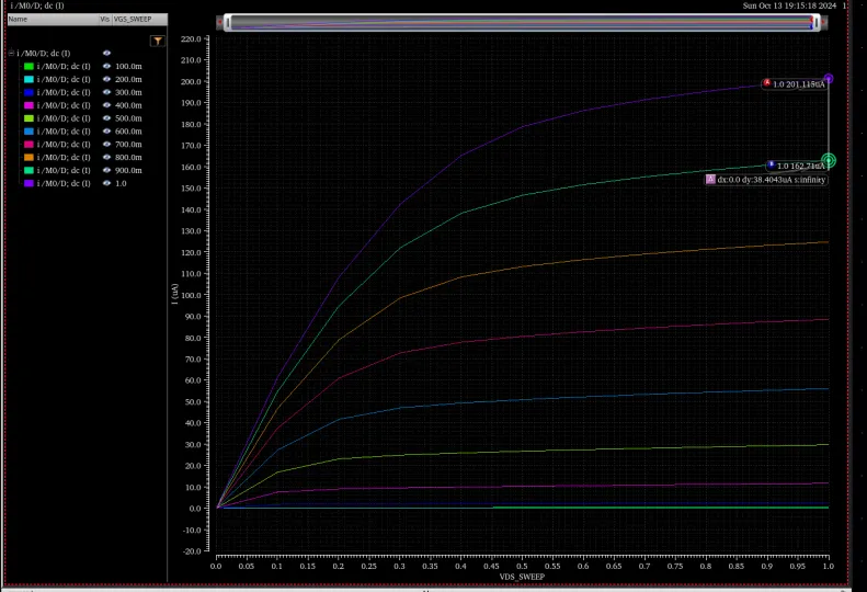
HW2-1c, p2 (35 points), restated from the key. Repeat part (a) for a device whose channel is 3.3 times longer ($L = 200$L= nm, the schematic’s l=200n). Estimate $v_{sat}$ by the same method, and explain why the answer differs from part (a).

Hint

The arithmetic is part (a)‘s. For the explanation: which condition must hold for the step formula to apply, and where does the length appear in it?

What it asks. Two things: the step method’s number for a channel 3.3 times longer, and why it differs from part (a). Most of the points are in the “why”. A saturation velocity belongs to electrons in silicon, not to one device, so the explanation has to be about the method, not about the carriers.

The idea. The number comes from part (a)‘s step method (Section 3) unchanged: $v = \Delta I_D/(C_{ox}W\,\Delta V_{GS})$ΔID​/(Cox​WΔVGS​). What is new is the condition behind its formula. $I_D = C_{ox}Wv_{sat}(V_{GS} - V_T)$ holds only when $(V_{GS} - V_T)/L \gg \mathcal{E}_{crit}/2$ (Chapter 4, Section 7), and $L$ sits in that condition. A longer channel at the same voltages has a weaker field, so it is less velocity-saturated, and the step it produces is a smaller share of $C_{ox}Wv_{sat}\Delta V_{GS}$Cox​Wvsat​ΔVGS​. The tempting explanation, the key’s, is that the longer device has a lower saturation velocity. It doesn’t: the two devices differ only in how far each is into velocity saturation.

The same step, from the readings on the key's plot

1. Read the top step at $V_{DS} = 1.0$ V, for part (a)‘s reasons: the top curves are the most saturated, and one $V_{DS}$ cancels the upward slope. Readings from the key’s plot: $201.115\,\mu\mathrm{A}$ at $V_{GS} = 1.0$ V and $162.71\,\mu\mathrm{A}$ at 0.9 V, so $\Delta I_D = 38.40\,\mu\mathrm{A}$ (Δ marker: 38.4043 µA).
2. Keep the denominator, because $W$W, $t_{ox}$ and the gate step haven’t changed: $C_{ox}W\,\Delta V_{GS} = 8.222\times10^{-12}\,\mathrm{C/cm}$10−12C/cm, as in part (a).
3. Divide, because a current is charge per length times velocity: $v = \dfrac{38.40\times10^{-6}}{8.222\times10^{-12}} = 4.67\times10^{6}\,\mathrm{cm/s}$106cm/s.
4. Compare with part (a), because the question asks why the two differ: $4.67/8.88 = 0.53$0.53.

Why it is lower. The saturation velocity is a property of electrons in silicon (Chapter 4, Section 1), about $10^7$ cm/s, the same in both devices. What changed is how far each device is into velocity saturation.

What the step method measures in each device

1. What the method assumes. It divides by $C_{ox}Wv_{sat}\Delta V_{GS}$Cox​Wvsat​ΔVGS​, which is the step only if $I_{DSAT} = C_{ox}Wv_{sat}(V_{GS} - V_T)$VT​). That holds only when $(V_{GS} - V_T)/L \gg \mathcal{E}_{crit}/2$ (Chapter 4, Section 7).
2. How far each device meets it. At the top of the family, with $V_T \approx 0.35$ V: $(1.0 - 0.35)\,\mathrm{V}/60\,\mathrm{nm} = 108$ kV/cm, against $\mathcal{E}_{crit}/2 \approx 12.5$ kV/cm with Chapter 4’s numbers: 8.7 times larger. At 200 nm it is $32.5$ kV/cm, only 2.6 times, because the same voltage is spread over a channel 3.3 times longer.
3. What that does to the current. The longer device is only partly velocity-saturated. Its current is $C_{ox}Wv_{sat}(V_{GS} - V_T)\frac{s - 1}{s + 1}$ with a smaller factor $\frac{s - 1}{s + 1}$s+1s−1​, so the step it produces is a smaller share of $C_{ox}Wv_{sat}\Delta V_{GS}$Cox​Wvsat​ΔVGS​.
4. What the number then means. Because the formula no longer fits the device, the step method returns an effective velocity, the average velocity of carriers that never fully reach $v_{sat}$vsat​, and not $v_{sat}$ itself.

In the widget above, the same model gives 67% of $v_{sat}$ at 60 nm and 46% at 200 nm: lower for the longer channel, as the homework found. Its numbers are not the simulator’s.

Check. Section 2’s length test is independent of this argument, and it agrees. The two velocities are in the ratio of the two steps, $8.88/4.67 = 1.90$1.90, and the top currents are in the ratio 2.29. Full velocity saturation in both devices would make both ratios 1; the square law would make them 3.33. Both lie in between, so the longer device is partly saturated, not a device with a lower ceiling. ✓

Answer: the method gives $4.67\times10^6$ cm/s, about half of part (a).

Remember. $v_{sat}$ belongs to the carriers, not to the device. When a longer channel gives a lower step-method number, say that the device is less velocity-saturated, so the method’s formula no longer fits; never that $v_{sat}$ fell.

The answer key differs

Its number agrees; its explanation doesn’t. It gives three reasons (p3) why the number differs:

1. the longer channel has fewer short-channel effects. Fair, if “short-channel effects” means velocity saturation;
2. “the electrical field across the channel is weaker …, thus, the saturation velocity … is lower”. The weaker field is the right cause, but the conclusion is wrong: the drift velocity is lower (the carriers don’t reach $v_{sat}$vsat​), while $v_{sat}$ itself is unchanged;
3. “there is also higher resistance with longer channel lengths, thus, the saturation velocity … is lower”. This doesn’t hold. A longer channel carries less current at the same overdrive, but that is the long-channel $1/L$ dependence, exactly what full velocity saturation removes. Resistance has no effect on $v_{sat}$vsat​.

So the result, $4.67\times10^6$ cm/s, should be read as “the step method no longer measures $v_{sat}$ for this device”, not as “this device has a lower $v_{sat}$vsat​”.

Check yourself A student fits the step method to three devices of the same process, L = 45, 90 and 500 nm, and gets 8.5, 7.0 and 2.5 × 10⁶ cm/s. What is the best estimate of v_sat, and what should the student say about the 500 nm number?

The shortest device is the most velocity-saturated, so 8.5×10⁶ cm/s is the best estimate, and still a slight underestimate: the fit approaches $v_{sat}$ from below as $L$ shrinks. The 500 nm device is mostly square-law at these voltages ($(V_{GS} - V_T)/L$(VGS​− is not much larger than $\mathcal{E}_{crit}/2$Ecrit​/2). Its 2.5×10⁶ cm/s is not a saturation velocity at all; the formula $C_{ox}Wv_{sat}(V_{GS} - V_T)$ doesn’t apply to it.

What this means for the midterm

Methods, and where the midterms use them.

• The subthreshold slope (part b): count decades, $\Delta V_{GS}/S$ΔVGS​/S; a smaller mV/decade is better. Every recent midterm asks it: MT24-2b and MT23-1b (leakage per µm from 10 µA/µm at $V_T$ and 90 mV/decade; M3, Section 1 and Section 2), and MT17-1c (the slope scales with temperature; M3, Section 9). About 8–10 points, 3–4 minutes. How to approach these is on M3’s device short-answer section.
• Velocity saturation against the square law (parts a and c): the transit-time delays assume a fully velocity-saturated device (MT21-2, M3, Section 8); M2’s chart says which model a question wants. The short answer is two sentences: current = charge × velocity; at high field the velocity is pinned at $v_{sat}$vsat​, so only the charge factor $C_{ox}(V_{GS} - V_T)$ is left. A past final asks the comparison directly (FN10-6, supply sensitivity of the delay under each model).
• Measuring $V_T$ (part b): name the definition (extrapolation at small $V_{DS}$VDS​, with $V_{DS}/2$VDS​/2; or a current criterion at $V_{DS} = V_{DD}$VDD​).

Traps.

• “Steeper” for a larger mV/decade. A larger number is a shallower, worse slope.
• Saying $v_{sat}$ changes with $L$L. It doesn’t; how saturated the device is does.
• Reading curves at different $V_{DS}$ in a family whose saturated curves still slope up.
• Rounding $C_{ox}$ early: 0.016 F/m² instead of 0.01644 moves the answer by 3%.

Time. On an exam, a step-method estimate from two given currents is a 3-minute part; the “why” is two sentences.

What the key gets wrong

All three numbers agree after re-solving. The disagreements are in the explanations; all are recorded in this page’s review/decisions.md.

Part	The key	Here
HW2-1b	100 mV/decade is “steeper” than 60	shallower, a worse slope; the reason it gives (more mV per decade) is right
HW2-1b (p3 note)	short devices “require an even lower mV” per decade	more mV per decade; the cause is $m > 1$1, poorer gate control in short devices
HW2-1b	$V_T$ “around 0.35–0.4 V”, read at the curve’s knee, no method	extrapolated intercept ≈ 0.36 V, so $V_T \approx 0.31$ V after the $V_{DS}/2$ correction; a ballpark either way
HW2-1c (p3 note)	the longer device’s “saturation velocity is lower”, from the weaker field and the higher resistance	$v_{sat}$ is unchanged; the longer device is less velocity-saturated, so the step method returns a lower effective velocity; resistance plays no part