22. Packaging and test: supply resonance, scan, stuck-at faults and reliability

Lecture 21 closes the course’s circuit topics by stepping outside the circuit: to the supply network that feeds the chip, the package that holds it, the tester that decides whether it works, and the years it must keep working afterwards. It opens with one more property of the supply network from Chapter 21: built to be quiet, it still has a resonance at a low frequency, the power-supply hum, and a program that switches a big block on and off at that frequency can bring a chip down. A brief tour of packaging follows: what a package does, the families from pin grid arrays to ball grid arrays, and why flip-chip bumps beat bond wires. The middle and heaviest part is design for test: why a fabricated die cannot be tested by running it, how a multiplexer in front of every flip-flop turns them into one long scan chain, how the stuck-at fault model turns “is this die good?” into a logic puzzle, and how a test pattern is found and run through the chain. The past finals test this part hardest. The lecture ends with reliability: the quiescent-current (I_DDQ) test, the bathtub curve, burn-in, the wear-out mechanisms that slow a chip as it ages, and built-in self-test.

After this chapter you can:

1. explain why the supply network resonates near $f_{clk}/10$fclk​/10, and what kind of activity excites it;
2. name a package’s functions and the main package families, and say why flip-chip bumps beat wire bonds;
3. tell design testing from acceptance testing, and say why functional testing does not scale;
4. draw a scan flip-flop and a scan chain, and give the scan test procedure with the order in which bits go in and come out;
5. find a test pattern for a stuck-at fault: control the node, sensitize a path, handle fan-out that reconverges, and count the patterns;
6. run a stuck-at test through a scan chain and say which scanned-out bit reveals the fault;
7. explain I_DDQ testing and the design rule it imposes;
8. read the bathtub curve, name an infant-mortality mechanism and say how burn-in exposes it, describe wear-out and its remedies, and tell ABIST from LBIST.

Boxes and equations marked board were written in the lecture. Parts marked added are explanations or examples this guide adds.

Symbols

Symbol	Meaning	Unit	First appears
$L$	the inductance of the supply’s path onto the chip (package, bond wires or bumps), lumped	nH	§1
$C$	the on-chip decoupling capacitance between $V_{DD}$ and ground, lumped	nF	§1
$R$	the series resistance of the supply path added	mΩ	§1
$f_{res}$fres​, $\omega$	the resonance frequency (Hz) and an angular frequency ($\omega = 2\pi f$ω=2πf, rad/s)	MHz, rad/s	§1
$Z(f)$	the impedance the chip’s current sees, looking into the supply network added	mΩ	§1
$f_{clk}$	the clock frequency	MHz, GHz	§1
$N$	the number of clock cycles between bursts of activity added	—	§1
SE	scan_enable: the select of the multiplexer in front of every scan flip-flop (1 = shift, 0 = normal)	—	§4
SI, scan_in	a scan flip-flop’s scan input; the chain’s input pin	—	§4
scan_out	the chain’s output pin: the last flip-flop’s Q	—	§4
D, Q, CLK	a flip-flop’s data input, output and clock (the board writes clk)	—	§4
$F_i$Fi​, $q_i$qi​, $D_i$	the $i$-th flip-flop of a chain, its state (Q), and the logic’s output that feeds its D added	—	§5
ST0, ST1	stuck at 0, stuck at 1 (the board’s abbreviations; other books write SA0, SA1)	—	§6
0/1	a node’s value in the good circuit / in the faulty circuit added	—	§6
$I_{DDQ}$	the supply current in the quiescent state (nothing switching)	mA	§9
$R_{short}$	the resistance of a defect from $V_{DD}$ to ground added	Ω	§9
$J$	current density in a wire, $I/(wt)$ added	mA/µm²	§10
$w$w, $w_{neck}$wneck​, $t$	a wire’s width, its width at a neck, its thickness	µm	§10
$V_{DD}$VDD​, $V_T$VT​, $\Delta V_T$	supply voltage, threshold voltage (its magnitude $\lvert V_T\rvert$ for a PFET), and a shift of the threshold	V, mV	§11, §12
$\tau$	a gate’s delay	ps	§12
$T$	the clock period	ps	§4, §12

1. Supply resonance: the power-supply hum

You need

Supply noise (Chapter 21). The chip’s current flows through the supply’s resistance and inductance, so the supply at the circuits droops by $IR$ (the DC part) and moves by $L\,dI/dt$ (the AC part, from the package’s and the network’s inductance).

Grids and decap (Chapter 21). Grids on every metal layer keep the network’s $R$ and $L$ low. Decoupling capacitance $C$ on the chip, between $V_{DD}$ and ground, supplies the fast current locally, so the transient does not have to come through the package’s inductance. Some decap comes free (metal–metal, the n-well, circuits that are not switching: implicit); the rest is built from MOS capacitors (explicit).

The supply’s path onto the chip (Chapter 21, Lecture20 @ 57:57, redrawn): the package’s inductance in each rail, and the decap beside the circuits. Original figure ↗

An LC tank added (circuits background). An inductor and a capacitor joined in a loop pass energy back and forth at the angular frequency $\omega = 1/\sqrt{LC}$1/LC​, that is at $f = 1/(2\pi\sqrt{LC})$ in hertz. Driven by a current at that frequency, the pair presents a large impedance, so a small current makes a large voltage; only the loop’s resistance limits it.

The question. Chapter 21 built the supply network to be quiet: low $R$ and $L$L, plenty of decap. Yet the package’s inductance and the chip’s decap are exactly an inductor and a capacitor. At what frequency do they ring, why does ordinary clocked activity leave the ring alone, and what kind of program can excite it?

The supply network is an RLC network

From a quiet network to a resonance (board, 01:35–04:42)

1. The recap board. The board at 01:35 restates Chapter 21: the power-supply network must reduce supply noise; low $R$ and $L$ (a grid); decoupling, implicit and explicit; the noise is $L\,dI/dt$LdI/dt.
2. A giant RLC network board. The network’s resistances, inductances and capacitances together form “a giant RLC network”, and “it has lots of one over the square root of LC resonances in it” (01:51). The board writes “RLC ⇒ $1/\sqrt{LC}$ resonances!” (02:45). If energy is put into the network at one of those frequencies, the supply noise is amplified.
3. One resonance always there board. The package’s inductance against the on-chip decap gives a resonance that sits, typically, near one tenth of the clock frequency: “resonance ≈ $\tfrac{1}{10}f_{clk}$ (low frequency)” (03:40). “This is often called power supply hum” (03:03).
4. Why it is usually harmless. A clocked chip draws its current in a burst at every clock edge. A pulse train at $f_{clk}$ has its energy at $f_{clk}$ and its harmonics ($2f_{clk}$2fclk​, $3f_{clk}$3fclk​, …), far above a resonance at $f_{clk}/10$fclk​/10: the clocking does not put energy into the hum (03:08–03:35).
5. The program that found it (03:35–04:40). Friends of the lecturer at AMD found chips failing on one particular piece of code: a loop that ran a floating-point multiply every 10 cycles. The multiplier is a high-power block; switching on once every ten cycles, it drew a burst of current that repeated at $f_{clk}/10$fclk​/10, exactly the hum. Such failures appear only with particular code, which is what makes them hard to find.

The supply network reduced to one loop added. The board supply $V_{DD}$ feeds the chip through the package’s resistance $R$ and inductance $L$ (here the loop’s total, both rails together). On the chip, the decap $C$ sits between the rails, and the switching logic draws a current $i(t)$i(t). $L$ and $C$ form a tank that rings at $f_{res}$ (the loop arrow).

The board (Lecture21 @ 04:42)

Lecture21 @ 04:42The supply network's recap, its 1/√(LC) resonances, and the hum near f_clk/10.

Fair copy of the board above (Lecture21 @ 04:42), mark for mark in its own layout, all in black: one pale cyan pen wrote the whole board. The middle, washed out by the striped shirt (the decoupling underline, “implicit”, “explicit”, and the dashed box round 1/√(LC) with its double arrow), is restored from 03:40; the double arrow and the bar under the ring are new at 04:42. “hum” and its quotes sit a little right of the board’s place, clear of the wider typeset “power supply”.

Putting numbers on the hum

The board gives only $1/\sqrt{LC}$ and “about $f_{clk}/10$fclk​/10”. Three added steps added make the picture quantitative.

The resonance frequency. The board’s $1/\sqrt{LC}$ is an angular frequency, in radians per second. In hertz, divide by $2\pi$2π.

The supply resonanceadded

$$f_{res} = \frac{1}{2\pi\sqrt{LC}}$$

Holds when: the package inductance L and the on-chip decap C treated as one lumped LC loop; the board writes the angular frequency 1/√(LC); a real network has many resonances, this is the lowest and strongest

Memorize it; the $2\pi$ is the usual slip.

The impedance the chip sees. Look into the supply from the chip’s current source. The decap $C$ is in parallel with the path back to the board, $R + j\omega L$jωL:

$$Z(f) = (R + j\omega L)\;\Big\|\;\frac{1}{j\omega C}, \qquad \omega = 2\pi f .$$

At low frequency the capacitor is an open circuit and $\lvert Z\rvert \to R$R. At high frequency the capacitor is a short and $\lvert Z\rvert \approx 1/(\omega C)$1/(ωC), falling. In between, at $f_{res}$fres​, the inductor’s and the capacitor’s reactances cancel in the parallel combination, and $\lvert Z\rvert$ peaks at about $L/(RC)$L/(RC): limited only by $R$R. A current component at frequency $f$ makes a supply ripple of that current times $\lvert Z(f)\rvert$∣Z(f)∣.

What excites it. A burst of activity every $N$ cycles repeats with period $N/f_{clk}$N/fclk​, so its current has a strong component at $f_{clk}/N$fclk​/N. The dangerous loop is the one with

$$N \approx \frac{f_{clk}}{f_{res}} .$$

Derive it: one repeat every $N$ cycles is a frequency of $f_{clk}/N$fclk​/N; set it equal to $f_{res}$fres​.

The impedance the chip sees added, computed from $Z(f) = (R + j2\pi fL)\,\|\,1/(j2\pi fC)$ with, for example, $L = 0.1$ nH, $C = 100$ nF and $R = 5$ mΩ. Flat at $R$ at low frequency, a peak of 202.5 mΩ at $f_{res} = 50.33$ MHz, then falling as $1/(2\pi fC)$1/(2πfC). The clock at 500 MHz sees 3.22 mΩ; a burst every ten cycles ($f_{clk}/10$fclk​/10, 50 MHz) lands on the peak.

A worked example: the hum of a 500 MHz chip (added; values for example)

1. The values. For example, $L = 0.1$ nH of package inductance, $C = 100$ nF of on-chip decap, $R = 5$ mΩ, $f_{clk} = 500$ MHz.
2. The resonance. $\sqrt{LC} = \sqrt{10^{-10} \times 10^{-7}}$ s $= 3.162$ ns, so $f_{res} = 1/(2\pi \times 3.162\ \text{ns}) =$ 50.33 MHz. Then $f_{clk}/f_{res} =$ 9.93: the hum sits at about $f_{clk}/10$fclk​/10, as the lecture says.
3. The impedance at the hum. Evaluating $Z$ at $f_{res}$ gives $\lvert Z\rvert =$ 202.5 mΩ. A quick estimate: $L/(RC) = 10^{-10}/(5\times10^{-3} \times 10^{-7}) = 200$ mΩ.
4. The impedance at the clock. At 500 MHz, $\lvert Z\rvert =$ 3.22 mΩ. A current component at the hum therefore makes 63 times the ripple of the same current at the clock frequency: 1 A of it would move the supply by 202.5 mV, a fifth of a 1 V supply, against 3.2 mV at $f_{clk}$fclk​. At DC, $\lvert Z\rvert = R = 5$ mΩ.
5. Which loop hits it. A burst every 10 cycles repeats at $500/10 =$ 50 MHz, where $\lvert Z\rvert =$ 201.8 mΩ: on the peak. A burst every 4 cycles repeats at 125 MHz, where $\lvert Z\rvert =$ 15.2 mΩ: well past it.

Check. Far above $f_{res}$ the capacitor carries almost all the current, so $\lvert Z\rvert \approx 1/(2\pi f C) = 1/(2\pi \times 5\times10^{8} \times 10^{-7}) =$ 3.18 mΩ at 500 MHz, close to the exact 3.22 mΩ (the small difference is the inductive branch in parallel).

More decap moves the hum; it does not remove it. Doubling $C$ lowers $f_{res}$ by $\sqrt2$ and halves the peak $L/(RC)$L/(RC). The hum is still there, at a different loop length.

Traps.

• $1/\sqrt{LC}$ in hertz. It is in radians per second; divide by $2\pi$2π, or the frequency comes out 6.28 times too high.
• “More decap removes the hum.” It moves it down as $1/\sqrt{C}$ and lowers the peak; a loop of a different length can still hit it.
• “A clocked chip’s current is at $f_{clk}$fclk​, whatever the code does.” A pattern of activity that repeats every $N$ cycles puts a component at $f_{clk}/N$fclk​/N.

Check yourself Why does a chip clocked at f_clk not normally excite a supply resonance at f_clk/10?

Its current comes in a burst at every clock edge, a periodic train at $f_{clk}$fclk​. Such a train has components only at $f_{clk}$ and its harmonics, all far above $f_{clk}/10$fclk​/10, where the network’s impedance is small. Only activity that itself repeats every ten or so cycles puts current at the hum.

Check yourself Double the decap in the worked example (C = 200 nF). Find the new resonance, and how often (in cycles) a burst must repeat to hit it.

$f_{res} = 1/(2\pi\sqrt{0.1\ \text{nH} \times 200\ \text{nF}}) =$ 35.59 MHz, lower by $\sqrt2$2​. A burst every $N$ cycles hits it when $N = f_{clk}/f_{res} = 500/35.59 =$ 14.05: about every 14 cycles. The peak falls to 102.5 mΩ (the estimate $L/(R \cdot 2C) = 100$ mΩ, half the 200 mΩ before), so the hum is weaker but still there.

Check yourself Does the hum's frequency depend on the clock frequency?

No: it is set by $L$ and $C$ alone. Only its ratio to the clock depends on $f_{clk}$fclk​, and that ratio is what decides which loop of code excites it.

2. Packaging (background for the final)

You need

Off-chip inductance (Chapter 21). The supply reaches the die through bond wires or bumps and the package’s leads, and each adds inductance in the supply path; so many are used in parallel, and decap is placed on the chip to supply the fast current locally.

The supply’s path onto the chip (Chapter 21, Lecture20 @ 57:57, redrawn): each $L$ is the package’s and its connections’ inductance. Original figure ↗

The question. What does a package do, what kinds are there, and why has the industry moved from wires bonded to the die’s edge to bumps over its whole face? This section is background for the final: no past final asks about packaging, so it is brief and has no worked example.

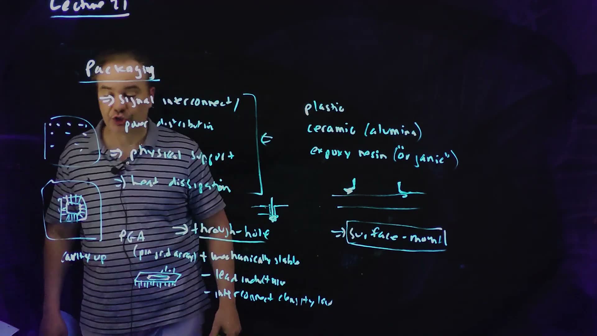
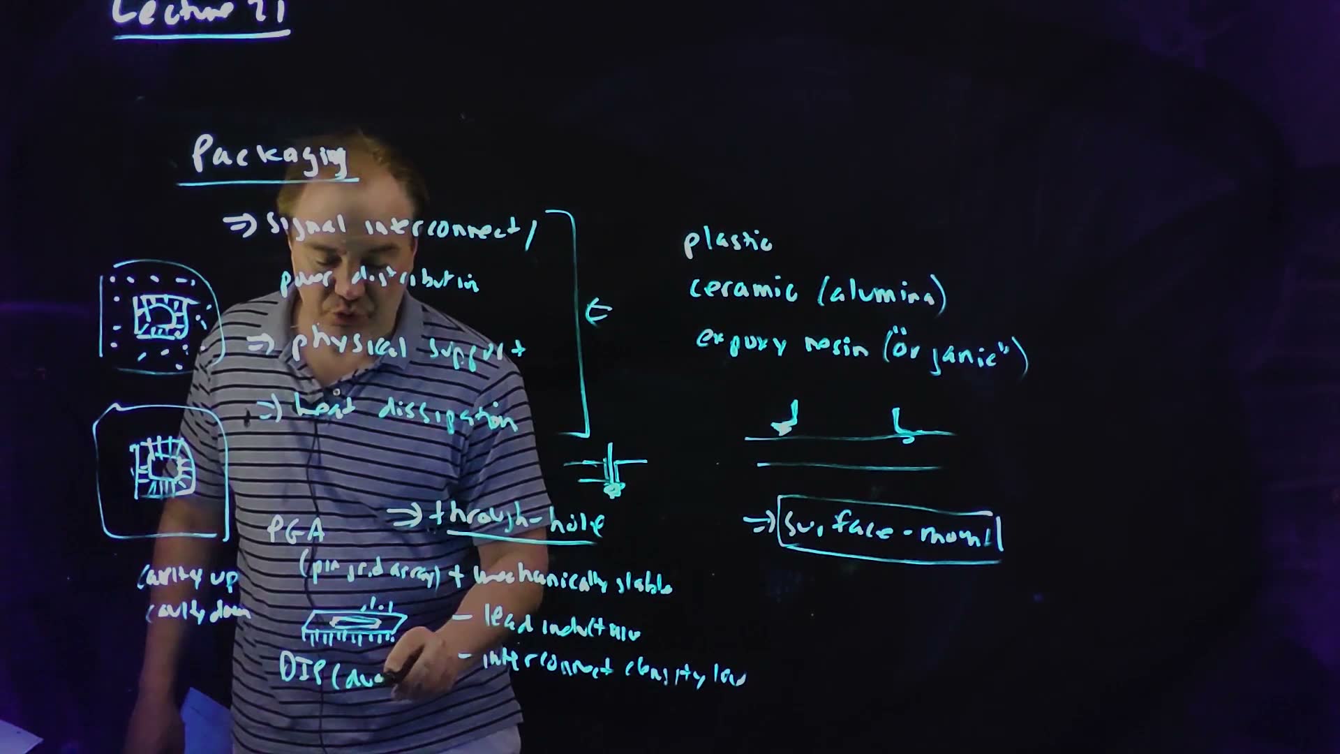
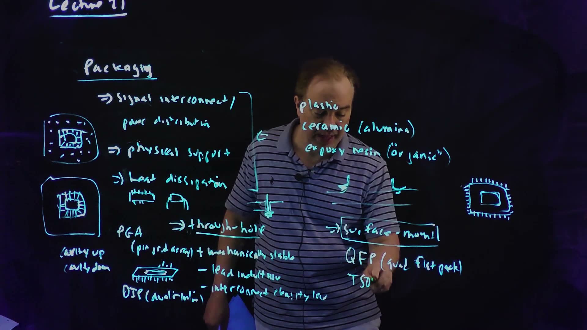
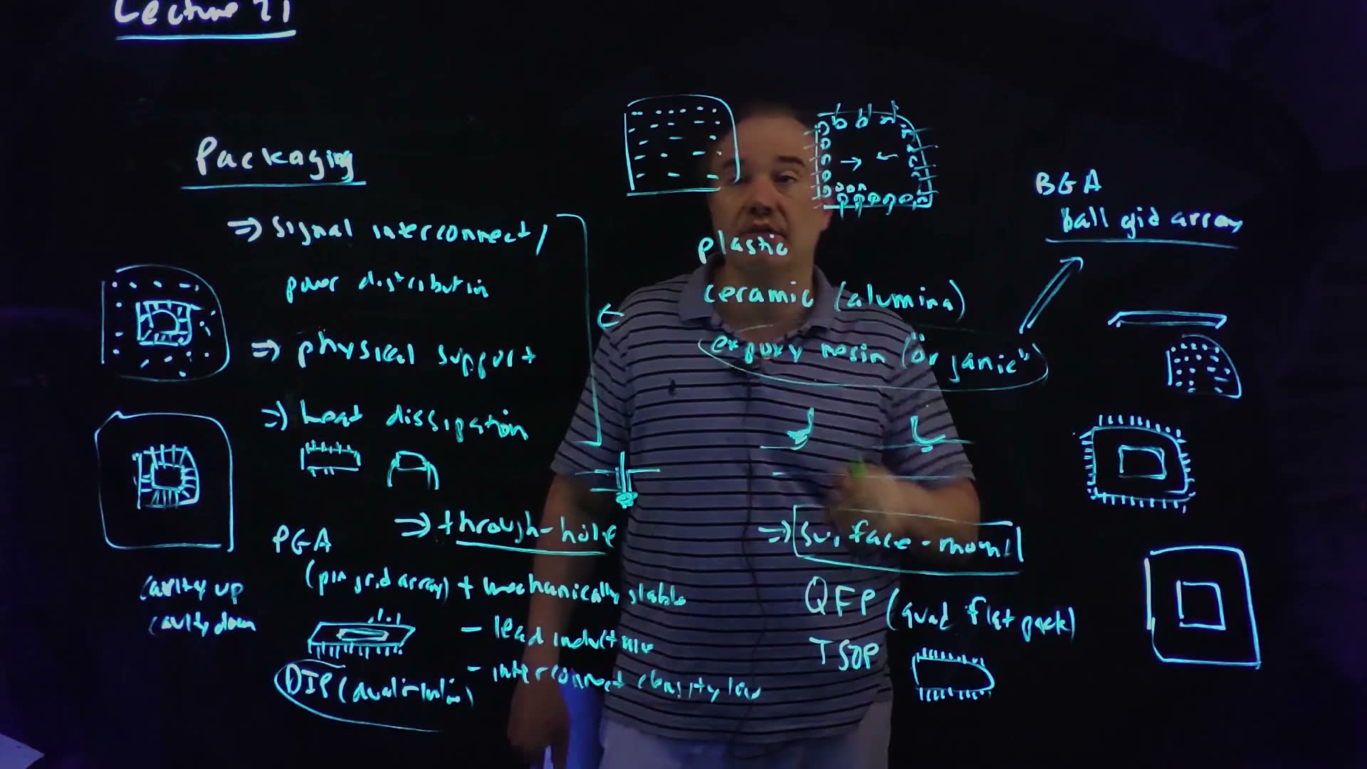
What a package does board (05:53). Three things: signal and power interconnect (one bracket on the board: the package carries both); physical support and protection; and heat dissipation.

What it is made of board (07:01): plastic; ceramic (alumina, Al₂O₃); and epoxy resin, called “organic”, the same family of material as FR4 circuit boards.

How it mounts on the board board (08:03–10:47).

• Through-hole: the leads pass through holes drilled in the board. It is mechanically stable, but the long leads add inductance and the interconnect density is low. Packages “through the mid-1990s were mostly through-hole packages” (08:11).
• Surface mount: the leads are soldered onto the board’s surface: lower inductance and higher density. Surface mount dominates today.

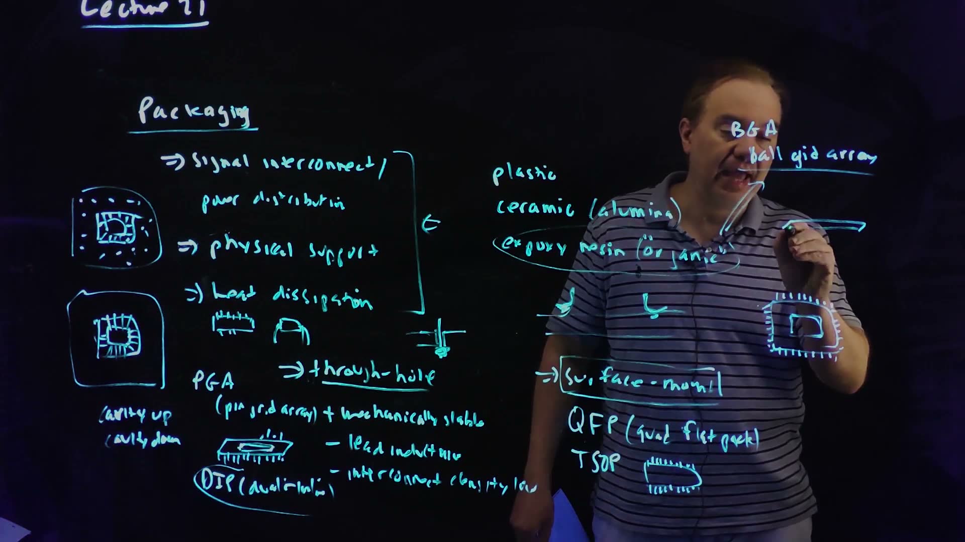
The families board (10:02–14:34).

• PGA, pin grid array (through-hole): pins in a grid under the package. The original Intel Pentium came in a ceramic PGA. Cavity up: the die faces up, wire bonded, pins below it. Cavity down: the die sits on the pin side and a heat sink goes on top, which cools better but leaves fewer pins for a given package size.
• DIP, dual in-line package (through-hole): two rows of leads, the package of the original TTL parts.
• QFP, quad flat pack (surface mount): leads on all four sides; microprocessors moved from PGAs to QFPs.
• TSOP, thin small outline package (surface mount): the usual DRAM package.
• BGA, ball grid array (surface mount): an organic substrate with an array of solder balls underneath, soldered to the board; the state of the art at the recording.

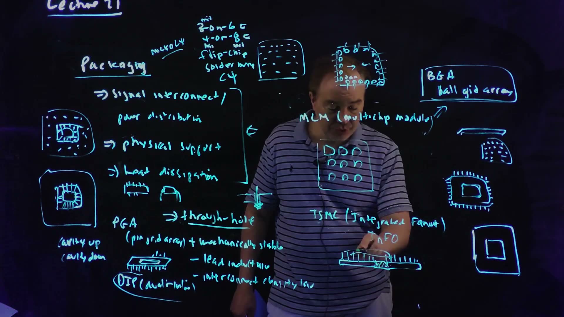
Inside a BGA: wire bond or flip-chip board (14:34–18:11).

• Wire bond. The die faces up, and bond wires run from pads in one or two rows around its periphery to the substrate. Bond wires “have a fair amount of inductance” (15:43), and the supply reaches the die’s centre only through its on-chip metal.
• Flip-chip. Solder bumps cover the whole face of the die, which is flipped face down onto the substrate. “Flip-chip”, “solder bump” and “C4” name the same joint (16:52). Bumps have far lower inductance than bond wires, far more connections fit, and power enters the die everywhere, including its centre.
• Bump sizes. “3-on-6 mil” means 3 mil bumps on a 6 mil pitch; “4-on-8 mil”, 4 mil bumps on 8 mil. A mil is a thousandth of an inch, 25.4 µm (“roughly 25 microns”), so 3-on-6 is about 75 µm bumps on a 150 µm pitch. Micro-C4 bumps are smaller still.

Several dies in one package board (19:18–22:16). A multichip module (MCM) puts several dies on one package: an old IBM RS/6000 module carried nine flip-chip dies on ceramic, as the lecturer recalls; MCMs are now built on organic substrates. TSMC’s InFO (integrated fan-out) goes further: the dies are embedded in a filler, and several layers of polyimide wiring, made lithographically, connect them and fan out to the bumps, with no package substrate at all. The result is thin and dense, which is why phones use it. Foundries are moving into packaging.

Three ways to package a die added, sketched after the boards (Lecture21 @ 14:34–22:16), same horizontal scale. (a) Wire bond on a BGA: bond wires from the die’s edge pads to the substrate. (b) Flip-chip on a BGA: the die face down on C4 bumps over its whole area; the larger BGA balls join the package to the board. (c) TSMC’s InFO: dies embedded in a filler with polyimide redistribution layers (RDL) beneath them and no substrate.

The board (Lecture21 @ 18:11)

Lecture21 @ 18:11The whole packaging board: functions, materials, through-hole and surface-mount families, BGA, flip-chip and the bump sizes.

Fair copy of the board above (Lecture21 @ 18:11), mark for mark in its own layout, all in black: one cyan pen wrote the whole board. The middle, behind the lecturer and his papers (plastic, ceramic (alumina), the epoxy oval, the two lead sketches, the left of the surface-mount box and QFP), is restored from 17:11, where it is clear; the box round BGA, the “mil” notes and the small c-marks after 3-on-6 and 4-on-8 are new by 18:11 and copied from it. The text is set smaller than the hand so that the crowded labels stay apart.

Traps.

• C4, flip-chip and solder bump are three names for one thing. A question that names one means all three.
• A BGA’s balls and a flip-chip’s bumps are different joints. The balls join the package to the board; the bumps join the die to the package. A flip-chip die usually sits in a BGA.
• Bumps win on inductance, not capacitance. The lecture once says “capacitance” (16:09); its point, made just before, is the bond wire’s inductance.

Check yourself Give two reasons a flip-chip die gets cleaner power than a wire-bonded one.

Each bump has far less inductance than a bond wire, so $L\,dI/dt$ is smaller; and bumps cover the whole die, so there are many more supply connections in parallel and power enters at the centre too, instead of crossing the die in on-chip metal from pads at the edge.

Check yourself About how many 3-on-6 mil bumps fit in one square millimetre, on a square grid?

The pitch is 6 mil $= 152.4$ µm, so a millimetre holds $1000/152.4 = 6.56$ bumps along each side: $6.56^2 \approx$ 43 per mm². With the lecture’s rounded 150 µm pitch, $6.67^2 \approx 44$44.

3. Design for test: what acceptance testing asks

You need

A synchronous machine (Chapter 13). Combinational logic sits between flip-flops, and one clock tells every flip-flop when to capture. What the logic computes depends on the inputs and on the flip-flops’ state, so the machine’s response to an input depends on its whole history.

Panel (a): logic between flip-flops on one clock (Chapter 13, added after Lecture12 @ 28:52). Original figure ↗

The question. A design has been simulated and fabricated. Thousands of dies come off each wafer, and some are bad. How does the manufacturer decide, die by die, which are good, how fast each one runs, and why it failed, in seconds per die?

From design testing to scan (board, 23:47–31:35)

1. Two kinds of testing board. Design testing asks whether the design meets its specification: simulation, what students do in their projects. Acceptance testing asks whether this fabricated die is good. Design for testability (DFT) is about the second (24:15).
2. Three questions board (25:33). For each die: does it work? Does it work at speed? And if not, what is the failure? The answers are a question of manufacturing yield: the fraction of dies that are good.
3. The tester. At the wafer level a tester applies patterns through a probe card, whose needles touch the die’s pads, then steps to the next die (25:29–26:37). Bad dies are discarded; Intel once set failed dies in Lucite as Christmas ornaments.
4. Speed sorting board (27:46). Identical dies run at different speeds, depending on the process corner each landed in. The tester measures each and bins it: the board’s 2.8, 3.0 and 3.2 GHz. The fast parts sell for more.
5. Functional testing does not scale board (28:31). The obvious test is to make the chip do things and check the results. Its test coverage is poor (“test coverage ✗”), and as chips grew, the tester time it needed became unmanageable.
6. Why not added. A response depends on the whole state. Take a modest block with 64 flip-flops and 32 inputs: it has $2^{64+32} = 2^{96} \approx$ 7.9 × 10²⁸ combinations of state and input. At a billion patterns a second, trying them all takes about 2.5 × 10¹² years. And a pattern cannot even be applied directly: the state must be reached by clocking the machine there.
7. The way out board (29:16–31:35). Scan-based testing: make every flip-flop’s state directly settable and readable (Section 4). Then the sequential problem becomes a combinational one, and test-generation tools keep the number of patterns small (Sections 6–7).

Acceptance testing at the wafer level added, after the board (Lecture21 @ 31:35). A probe card touches one die’s pads; the tester (automatic test equipment, ATE) applies patterns and reads the responses; a bad die is marked for discard (✗) and a good one is binned by its measured speed (the board’s 2.8, 3.0 and 3.2 GHz). Then the prober steps to the next die.

The board (Lecture21 @ 31:35)

Lecture21 @ 31:35The whole design-for-test board: design versus acceptance testing, the three questions, speed sorting, functional testing and scan.

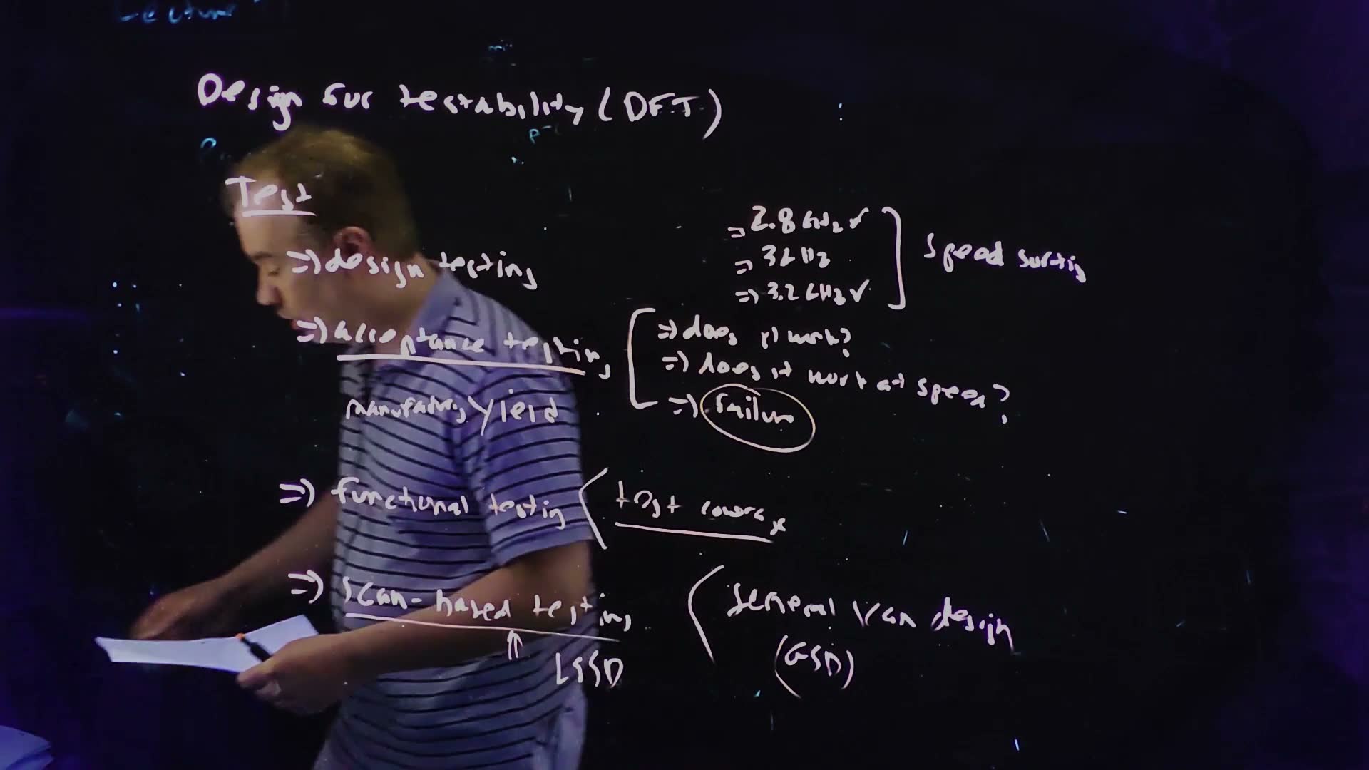
Fair copy of the board above (Lecture21 @ 31:35), mark for mark in its own layout, all in black: one pale pink-white pen wrote the whole board. The starts of “design testing” and “acceptance testing”, behind the lecturer, are restored from 30:39. The faint remnant of “Lecture 21” at the top left is left out.

Traps.

• Design verification is not acceptance testing. A design that passes every simulation still yields bad dies; acceptance testing finds them.
• “It works” is not “it works at speed”. A die can compute every answer right at a slow clock and fail at the rated one; at-speed testing (Section 5) is a separate question.
• Speed bins are not different designs. The same mask set gives dies of different speeds; testing sorts them.

Check yourself Which of the three acceptance questions does speed sorting answer?

“Does it work at speed?”, asked at several speeds: each die is binned at the fastest clock at which it still works.

Check yourself Add 32 flip-flops to step 6's block. By what factor does the number of combinations grow, and how long would trying them all take now, at a billion patterns a second?

Each extra flip-flop doubles the count, so it grows by $2^{32} \approx$ 4.3 × 10⁹, to $2^{128}$2128. The time grows by the same factor: $2.5 \times 10^{12} \times 4.3\times10^{9} \approx$ 1.1 × 10²² years.

4. The scan flip-flop and the scan chain

You need

The edge-triggered flip-flop (Chapter 13). Two latches in series on opposite clock phases make a flip-flop: when the first (the master) closes, the second (the slave) opens and shows what the master caught. The active edge is the edge at which the master closes. Chapter 13’s drawing has the master on clk (transparent while clk = 1), so it captures at the falling edge; swapping the phases (master transparent while clk = 0, slave while clk = 1) gives a positive-edge flip-flop, which captures at the rising edge. Each latch is static: it holds its value through a pair of inverters whose loop a clocked switch closes (Chapter 13).

A master–slave flip-flop (Chapter 13, Lecture12 @ 56:32, redrawn): master on clk, slave on clk̄, so it captures at clk’s falling edge. Swap clk and clk̄ for the positive-edge flip-flop this chapter uses. Original figure ↗

A 2:1 multiplexer (Chapter 10). A multiplexer passes one of two inputs to its output, chosen by a select. Built from two transmission gates, one driven by the select and one by its complement, it is static because exactly one gate is on at a time (the selects are one-hot).

The long-path constraint (Chapter 13). Data launched at one rising edge must pass the launching flip-flop and the logic and arrive a setup time before the next edge: $t_{clk\to Q} + t_{logic} + t_{setup} \le T$T, where $T$ is the clock period.

The question. Section 3 needs every flip-flop’s state to be settable and readable from outside the chip, but a chip has thousands of flip-flops and a few hundred pins. How can every flip-flop be reached through two pins?

A multiplexer in front of every flip-flop

The scan pair (board, 32:07–33:30)

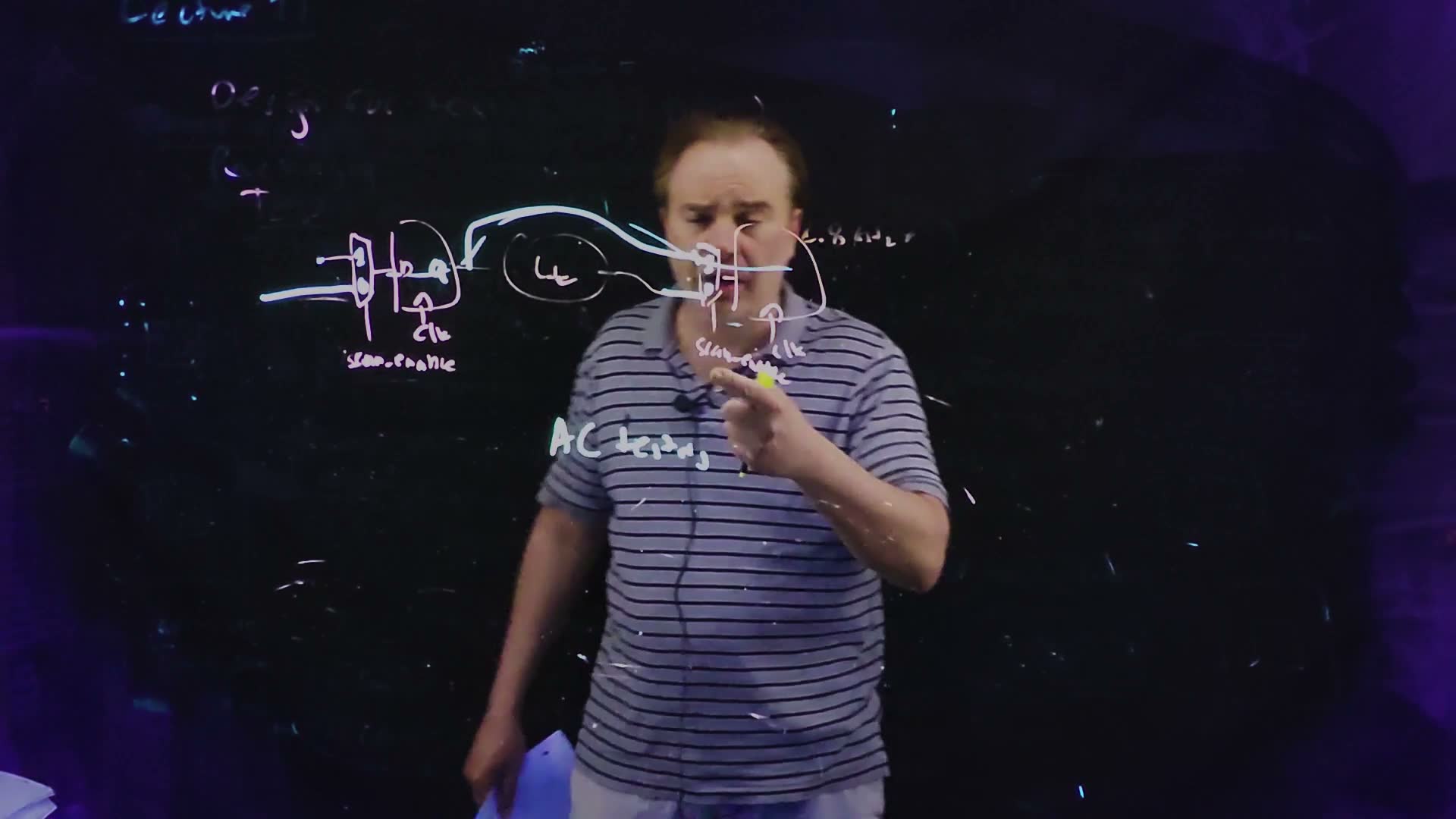
1. The mux board. In front of each flip-flop’s D input, put a 2:1 multiplexer. Its select is scan_enable (SE). Its input 0 takes the combinational logic’s output, the normal D. Its input 1 takes the previous flip-flop’s Q (32:07–33:16).
2. SE = 0: normal operation. Every mux passes its logic input, and the circuit is exactly the original: logic between flip-flops.
3. SE = 1: one giant shift register. Every mux passes its neighbour’s Q, so at each clock edge every flip-flop takes the value of the one before it. The flip-flops form one long shift register, the scan chain, from a scan_in pin into the first flip-flop to a scan_out pin from the last.

Two scan flip-flops with logic between them, redrawn from the board (Lecture21 @ 33:30). Each flip-flop’s D comes from a 2:1 multiplexer whose select is SE (the board’s scan_enable): input 0 is the logic (the oval, the board’s “c.l.” for combinational logic), input 1 is the previous flip-flop’s Q (the thick arc). With SE = 1 the arc carries the first flip-flop’s state straight into the second.

The board (Lecture21 @ 33:30)

Lecture21 @ 33:30The scan pair: a multiplexer on scan_enable in front of each flip-flop, the shift path arcing over the logic.

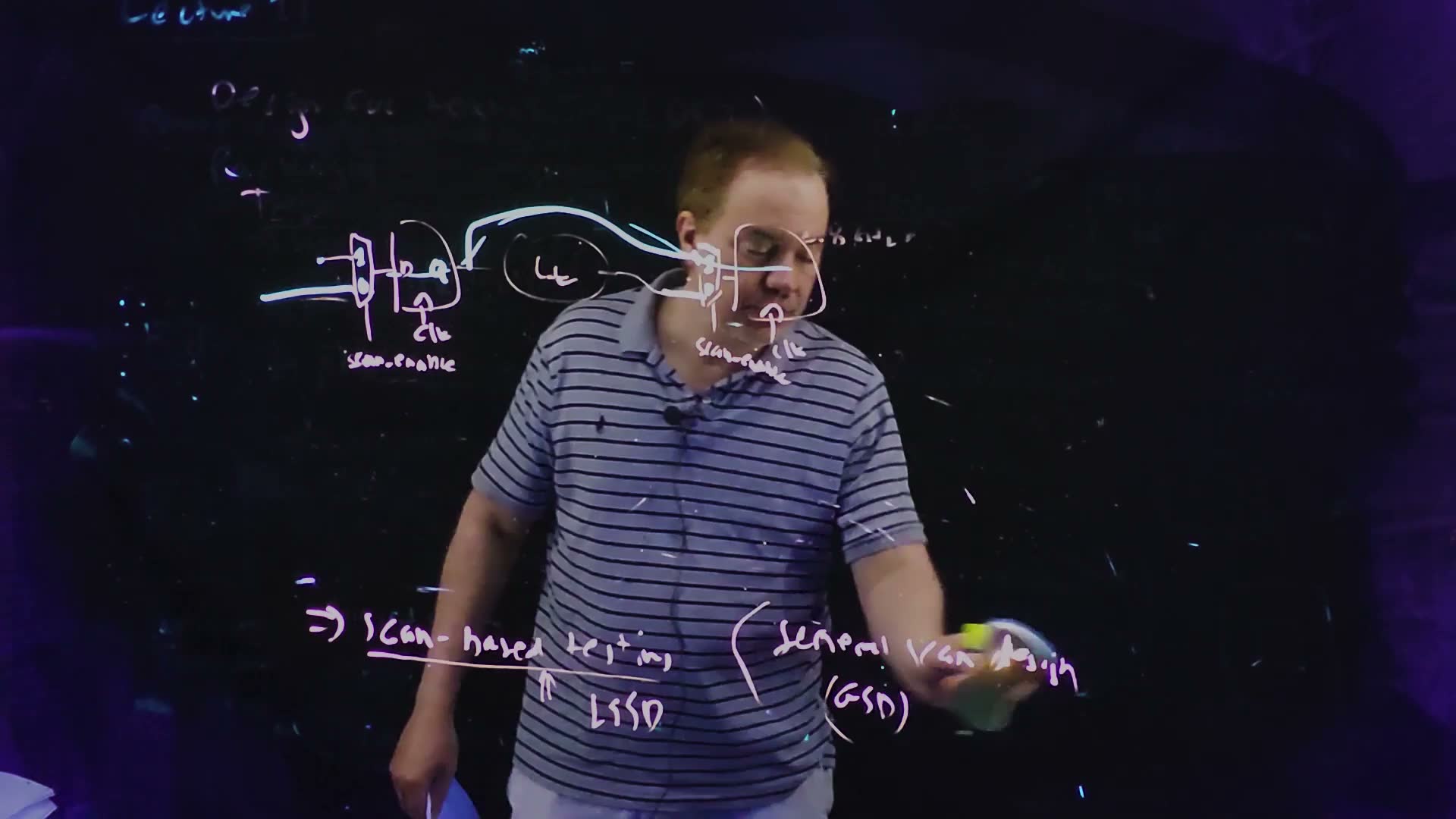
Fair copy of the board above (Lecture21 @ 33:30), mark for mark in its own layout, all in black: one pale pink-white pen; the heavy arc and the heavy input line are a fresh marker in the same layer, drawn heavier. Faint remnants of the erased design-for-test board are grey. The second multiplexer and flip-flop, behind the lecturer’s head, are restored from 34:15. The oval’s label, written like “Lc”, marks the combinational logic.

A three-flip-flop scan chain added, in its two modes. Each box is a scan flip-flop (the mux and the flip-flop together), with inputs D, SI, SE and CLK. (a) SE = 1: the flip-flops form a shift register from scan_in through $F_1$F1​, $F_2$F2​, $F_3$ to scan_out (thick); the logic is ignored. (b) SE = 0: the circuit runs normally; each flip-flop takes its $D_i$ from the logic (thick), which reads the states $q_1$q1​, $q_2$q2​, $q_3$ and the primary input $P$P.

The scan flip-flop as one cell

Problem sets and finals draw a scan flip-flop as one box with four inputs added: D, SI (scan in), SE and CLK. Its function, at each rising edge of CLK:

The scan flip-flopadded

$$Q^{+} = \overline{SE}\cdot D \;+\; SE\cdot SI$$

Holds when: a positive-edge flip-flop with a 2:1 mux on SE in front of its D; SE and the selected input stable for setup and hold around the edge; Q changes only at the rising edge

Memorize it: SE = 0 takes D, SE = 1 takes SI, and nothing changes between rising edges.

How it is built, at gate level as the board draws it (33:30): the 2:1 multiplexer on SE, then a positive-edge master–slave flip-flop, Chapter 13’s pair with its phases swapped. The mux can be the transmission-gate pair of Chapter 10, driven by SE and $\overline{SE}$SE; each latch holds its value through a feedback inverter pair closed by a clocked switch, so the cell is static.

The scan flip-flop at gate level, as the board draws each scan cell (Lecture21 @ 33:30). A 2:1 multiplexer on SE passes D (input 0) while SE = 0 and SI (input 1) while SE = 1 into the D input of a positive-edge flip-flop, which copies it to Q at each rising edge of CLK. Inside the box is Chapter 13 §10’s master–slave pair with its phases swapped.

A worked example: one rising edge through the cell (added)

1. Before the edge (CLK = 0), SE = 1, D = 0, SI = 1. The mux passes SI, so its output is 1. The master is transparent and follows it: the master holds 1. The slave is closed: Q keeps its old value, say 0.
2. The rising edge. The master closes on 1; the slave opens and passes it: Q = 1.
3. CLK = 1, D and SI change. The master is closed, so nothing it sees reaches Q: Q stays 1.
4. The falling edge, now with SE = 0. The master opens again and follows the mux, which now passes D = 0; the slave closes, holding Q. Q stays 1 until the next rising edge, which brings in 0.

So the cell changes Q only at a rising edge, to SI if SE was 1 and to D if SE was 0: the formula above.

Where scan came from, and what it costs

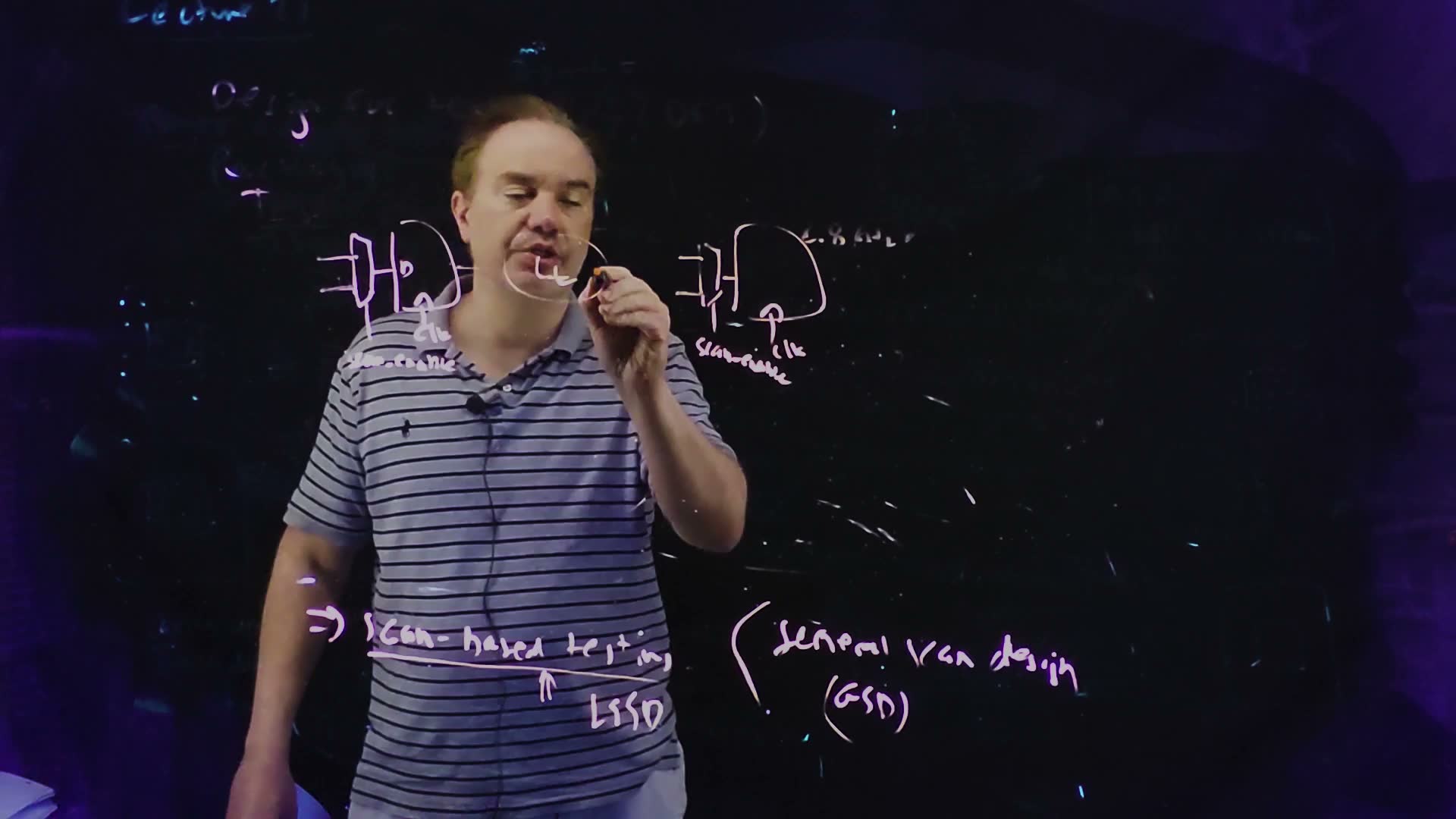
LSSD and general scan design board (29:39–31:31). IBM pioneered scan as LSSD, level-sensitive scan design: every flip-flop was scannable, with strict clocking rules, and “if you broke the rules, they would send you to Burlington to take a class” (31:02). The industry’s general scan design (GSD) is looser. It allows a designer to leave scan off some flip-flops, for performance, as long as the test tools can still generate patterns around them.

The cost added. The mux sits in every flip-flop’s data path, so its delay adds to the long path: $t_{clk\to Q} + t_{logic} + t_{mux} + t_{setup} \le T$T. There is also the mux’s area, and the SE and SI wires to route. That is why GSD lets designers drop scan on the most critical flip-flops.

Traps.

• The mux’s polarity. SE = 1 must select SI (the shift path); the board marks the shift input “1”. Swapped, the chain shifts in normal operation.
• Changing SE at a clock edge. SE selects the data path, so it must be steady for setup and hold around each edge, like D. Waveforms change SE between edges.
• “Scan replaces the flip-flop.” It is the same flip-flop with a multiplexer in front; in normal operation the circuit is unchanged.

Check yourself In the scan cell, which input does SE = 1 select, and why must the two selects of a transmission-gate mux be one-hot?

SE = 1 selects SI, the previous flip-flop’s Q (the shift path). The two transmission gates are driven by SE and $\overline{SE}$SE, so exactly one is on: if both were on, D and SI would fight at the mux output; if neither, the output would float and the cell would not be static.

Check yourself For example, a path has 400 ps of logic, t_clk→Q = 50 ps and t_setup = 30 ps, and the scan mux adds 40 ps. What is the minimum clock period before and after scan is added, and by what fraction does the fastest clock fall?

Before: $50 + 400 + 30 =$ 480 ps. After: $480 + 40 =$ 520 ps. The fastest clock falls from 2.083 GHz to 1.923 GHz, by 7.7 %: the price of making this flip-flop scannable, and the reason GSD may drop scan on it.

Check yourself What does LSSD require that general scan design does not?

That every flip-flop be scannable, under strict clocking rules. GSD lets a designer leave some flip-flops off the chain for speed, provided the test tools can still cover the logic around them.

5. The scan test: shift in, capture once, shift out

You need

The scan chain (Section 4). Each flip-flop has a 2:1 multiplexer in front of D, selected by SE. At each rising edge, $Q^{+} = \overline{SE}\cdot D + SE\cdot SI$SI. With SE = 1 the flip-flops form a shift register from scan_in through $F_1, F_2, \ldots, F_n$ to scan_out (scan_out is $F_n$‘s Q); with SE = 0 each $F_i$ takes $D_i$ from the logic.

The three-flip-flop scan chain in its two modes (Section 4). Original figure ↑

The question. With the chain in place, what exactly does the tester do, clock by clock, and in what order do the bits go in and come out?

The procedure

One scan test (spoken, 33:16–34:53)

1. Shift in (SE = 1). Shift the desired state into the chain, one bit per clock edge: $n$ edges for $n$ flip-flops.
2. Capture (SE = 0). Apply the primary inputs, and give one clock edge: every flip-flop captures the logic’s output, $D_i$Di​.
3. Shift out (SE = 1). Shift the captured state out through scan_out, $n$ edges, and compare it with the good circuit’s response. The next pattern shifts in through scan_in at the same time.

Why it works. Every flip-flop is now directly controllable (its state is set by shifting in) and directly observable (its captured value is read by shifting out). The tester no longer has to drive the machine through a sequence of states to reach a test: one pattern tests the combinational logic between the flip-flops, from known inputs to observed outputs. “And this is the beauty of scan-based testing” (34:53). What remains is to choose a small set of patterns (Sections 6–7).

The order: first in, farthest along

The lecture states the procedure; the bit order follows from the wiring added, and the finals ask for it.

• Loading. Each shift edge moves every bit one place along, so the first bit shifted in travels farthest. To load $q_1 q_2 \ldots q_n$q1​q2​…qn​, put $q_n$ on scan_in first and $q_1$ last.
• Unloading. scan_out is $F_n$‘s Q. Right after the capture edge it already shows $F_n$‘s captured value, $D_n$Dn​. Each shift edge then brings the next: $D_{n-1}$Dn−1​, …, $D_1$D1​.

The bit order in a scan chainadded

$$\begin{aligned} \text{scan\_in, in time order:}\quad & q_n,\ q_{n-1},\ \ldots,\ q_1 \\ \text{scan\_out, in time order:}\quad & D_n,\ D_{n-1},\ \ldots,\ D_1 \end{aligned}$$

Holds when: a chain scan_in → F1 → … → Fn → scan_out; SE = 1 for the shifts; scan_out is Fn's Q

Derive it, every time, from one shift: “the bit that goes in first is pushed farthest along; the bit nearest the output comes out first”.

A worked example: the chapter’s own circuit

An added example added, used again in Section 8. A chain scan_in → $F_1$ → $F_2$ → $F_3$ → scan_out, a primary input $P$P, and the logic

$$\begin{aligned} G &= \overline{q_1 + q_2}\ (\text{NOR}), & D_1 &= \overline{G\,q_3}\ (\text{NAND}), \\ D_2 &= \overline{G + P}\ (\text{NOR}), & D_3 &= q_1 q_3\ (\text{AND}). \end{aligned}$$

The chapter’s example circuit added: a three-flip-flop scan chain with its logic opened. $G = \mathrm{NOR}(q_1, q_2)$NOR(q1​,q2​); $D_1 = \mathrm{NAND}(G, q_3)$NAND(G,q3​); $D_2 = \mathrm{NOR}(G, P)$NOR(G,P); $D_3 = \mathrm{AND}(q_1, q_3)$AND(q1​,q3​), with $P$ a primary input. The small cross on $G$ is the fault site of Section 8.

Load 001, capture with P = 0, unload

1. What to shift in. We want $q_1q_2q_3 = 001$001. The first bit in ends in $F_3$F3​, so scan_in carries $q_3, q_2, q_1$ = 1, 0, 0, one per shift edge.
2. The chain after each load edge. $(q_1, q_2, q_3)$ = (1, –, –), then (0, 1, –), then (0, 0, 1): the target (– is whatever was there before).
3. Capture, with SE = 0 and $P = 0$0. $G = \overline{0 + 0} = 1$1; $D_1 = \overline{1 \cdot 1} = 0$0; $D_2 = \overline{1 + 0} = 0$0; $D_3 = 0 \cdot 1 = 0$0. The capture edge loads $(D_1, D_2, D_3)$ = (0, 0, 0).
4. Unload. scan_out shows $D_3 = 0$ at once, then $D_2 = 0$ after the first shift edge and $D_1 = 0$ after the second: 0, 0, 0.

The whole test takes seven clock edges: three to load, one to capture, three to unload.

At-speed testing

AC testing, or at-speed testing board (35:24–35:50): shift a state in slowly, then give the capture edge at the target clock period after the edge that launches the logic’s inputs. A path too slow for that period captures a wrong value in a known flip-flop. The test then not only says the die is slow; it names the flip-flop at the end of the failing path. (The lecture’s spoken “don’t need timing” is “don’t meet timing”.)

The waveforms

The procedure drawn on one time axis added. SE changes only midway between clock edges; it is high for the three load edges L1–L3, low across the capture edge C, and high again for the unload edges U1–U3.

The scan test of the example circuit, cycle by cycle added, computed from the shift-register simulation (the guide’s scan.ts) for the load $q_1q_2q_3 = 001$ and $P = 0$0. SE changes only between edges. scan_in carries 1, 0, 0 into the load edges L1–L3; after L3 scan_out shows the loaded $q_3 = 1$1. The capture edge C loads $(D_1, D_2, D_3)$(D1​,D2​,D3​), and scan_out shows $D_3$ at once, then $D_2$ after U1 and $D_1$ after U2. Hatching marks values that do not matter. The last row, the faulty circuit’s scan_out, belongs to Section 8: the two bits marked ≠ differ from the good row.

Traps.

• Shifting the pattern in the written order. Putting $q_1, q_2, q_3$ on scan_in in that order loads it reversed.
• Counting the first scan_out bit after the first shift edge. $D_n$ is on scan_out as soon as the capture edge has passed; the first shift edge brings $D_{n-1}$Dn−1​.
• Leaving SE = 1 across the capture edge. The chain just shifts once more and the logic is never sampled.
• “The primary inputs are scanned.” They are not flip-flops: the tester applies them directly, and they must be steady around the capture edge.

Check yourself To load q1q2q3 = 110 into the example chain, what goes on scan_in, in time order?

The first bit in ends in $F_3$F3​, so $q_3$ goes first: 0, 1, 1. After the first edge the chain holds (0, –, –); after the second, (1, 0, –); after the third, (1, 1, 0).

Check yourself How many clock edges does one complete test of a 3-flip-flop chain take? How many do ten tests take when each pattern's shift-in overlaps the previous shift-out?

One test alone: $3 + 1 + 3 =$ 7 edges. Overlapped, each pattern costs 3 shift edges and 1 capture edge, and the last result needs 3 more to come out: $10 \times 4 + 3 =$ 43 edges, against $10 \times 7 = 70$ without overlap.

Check yourself What does an at-speed capture tell you that a slow capture cannot?

Whether the logic meets the rated clock period. A slow capture gives every path plenty of time, so it finds only logic faults; an at-speed capture finds paths too slow for the clock, and the flip-flop that captured a wrong value names where the slow path ends.

6. Fault models: stuck-at-0 and stuck-at-1

You need

What scan leaves (Section 5). Through the scan chain every flip-flop’s state can be set and read, so testing the chip becomes testing its combinational logic: apply a pattern to the logic’s inputs (the scanned states and the primary inputs) and read its outputs.

Gate truth tables. A NAND’s output is 0 only when all its inputs are 1; a NOR’s output is 1 only when all its inputs are 0; an AND’s output is 1 only when all inputs are 1; an OR’s is 0 only when all are 0.

The scan chain (Section 4): panel (b) is the logic each pattern tests. Original figure ↑

The question. A defect can be a short, an open, a particle, a bad contact: endlessly many physical things. What single, simple description of “something is wrong” can a program generate tests for?

From defects to a fault model (board, 36:40–41:06)

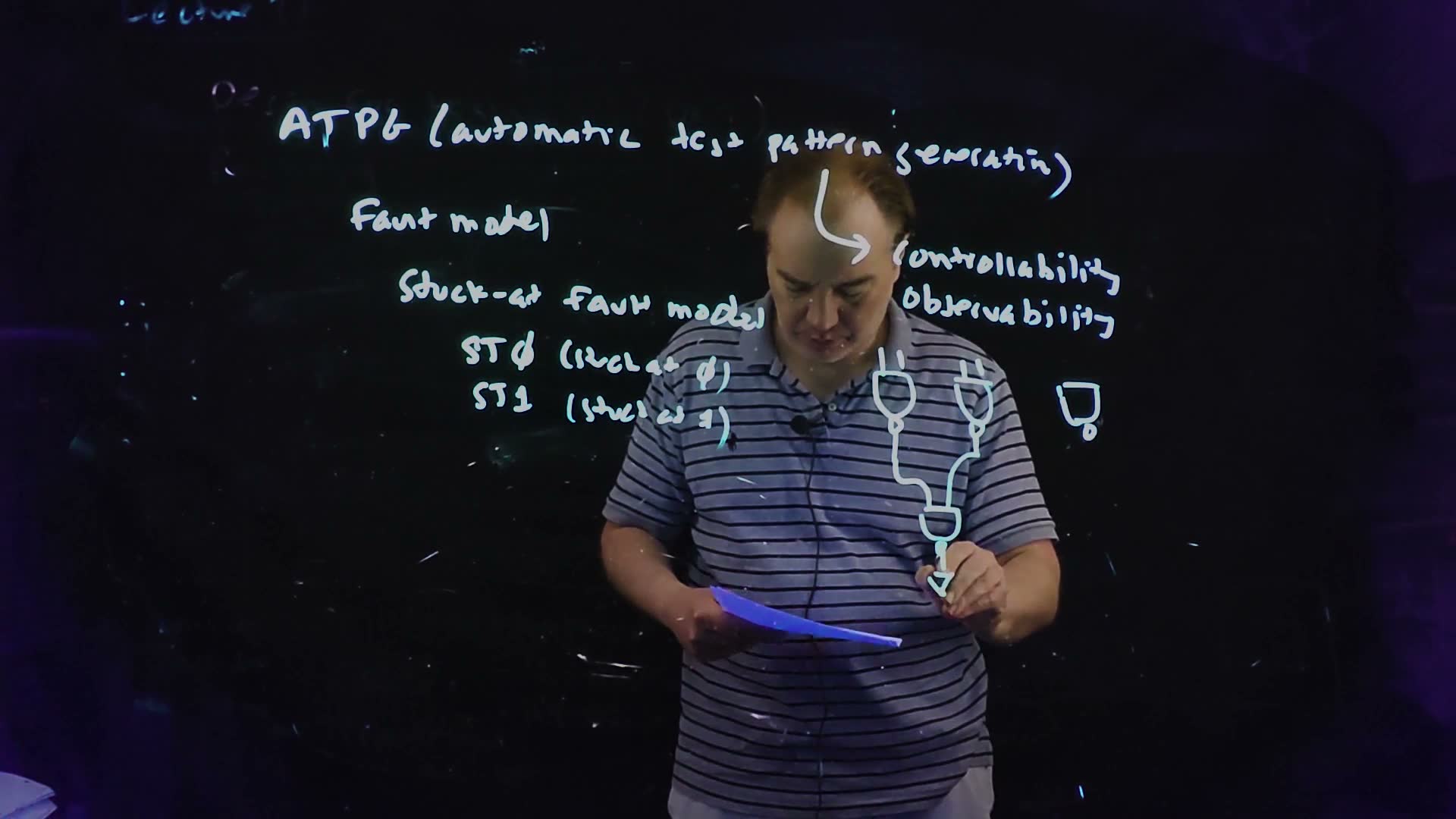
1. ATPG board. Test patterns come from automatic test pattern generation tools (37:35): FastScan, from Mentor Graphics at the time, and in-house tools at most companies.
2. A fault model board (39:18). To generate patterns, the tool needs a fault model: a description of how a physical defect shows up in the logic.
3. The stuck-at model board. “No matter what the fault is, short, open, whatever it is, the way it’s manifest is that a … node in your logic network is stuck at either a zero or a one” (38:09). The board writes ST0 (stuck at 0) and ST1 (stuck at 1). It has been criticized for decades and never replaced. It is applied at the logic level, to the gate netlist, not to the transistors (41:06).
4. Picturing it added. A node shorted to $V_{DD}$ reads 1 whatever drives it: ST1. Shorted to ground: ST0. A gate input cut off from its driver floats, and often settles at one value, acting as stuck at 0 or at 1. Each node can fail two ways, so a netlist with $n$ nodes has $2n$ single stuck-at faults.
5. What a test is added. A pattern detects a fault if the good circuit and the faulty one give different outputs for it. To keep both in view, write a node’s value as good/faulty: 0/1 means “0 in the good circuit, 1 in the faulty one”.

Three defects and the faults they look like added. (a) Node $n$ shorted to $V_{DD}$VDD​: whatever the inverter drives, $n$ reads 1, stuck at 1. (b) Shorted to ground: stuck at 0. (c) An open: the NAND’s input is cut from its driver and floats; it often settles at one value and behaves as stuck at 0 or stuck at 1.

A worked example: the faults of one NAND

An added example added, by exhaustive simulation. A 2-input NAND, inputs $a$ and $b$b, output $y$y, has six single stuck-at faults. For each, which input patterns $ab$ detect it?

Six faults, four patterns

1. $y$ ST1. The faulty output is always 1, so a pattern detects it only where the good output is 0: 11 alone.
2. $y$ ST0. Detected where the good output is 1: 00, 01, 10.
3. $a$ ST0. The faulty NAND sees $a = 0$0, so its output is 1. The good output must be 0, which needs $a = b = 1$1: 11 alone. $b$ ST0 is the same: 11.
4. $a$ ST1. We need $a = 0$ in the good circuit (opposite to the stuck value) and the change to reach $y$y, which needs $b = 1$ (a 0 on $b$ would force $y = 1$ either way): 01 alone. By symmetry, $b$ ST1: 10.
5. The smallest covering set. $a$ ST1 needs 01, $b$ ST1 needs 10, and the stuck-at-0 inputs need 11; those three also cover both output faults. So $\{11, 01, 10\}${11,01,10}, three of the four patterns, tests all six faults, and no smaller set does. The pattern 00 detects only $y$ ST0, which 01 and 10 already detect.

Traps.

• “A stuck-at test proves the transistors are right.” It is a logic model: a defect that slows a gate or draws extra current without changing a logic value escapes it. At-speed tests (Section 5) and I_DDQ tests (Section 9) catch some of those.
• “Stuck-at 1” is not “the node is 1 in this pattern”. It means the node is 1 in every pattern, in the faulty circuit; to see it, the pattern must make the good node 0.

Check yourself Which input patterns of a 2-input NOR detect its output stuck at 0?

Only where the good output is 1, which for a NOR is 00 alone.

Check yourself How many single stuck-at faults does a 2-input NOR have, and what is its smallest pattern set covering them all?

Three nodes, two faults each: 6. By the NAND’s argument with the values inverted: an input stuck at 1 needs both inputs 0 (00); input $a$ stuck at 0 needs $a = 1$1, $b = 0$ (10); $b$ stuck at 0 needs 01. These three also cover both output faults: the set $\{00, 10, 01\}${00,10,01}.

7. Controllability and observability: finding a test pattern

You need

The stuck-at model (Section 6). A fault is one node stuck at 0 (ST0) or at 1 (ST1); a pattern detects it if the good and faulty circuits’ outputs differ. A node’s value is written good/faulty, e.g. 0/1.

Controlling values added. A 0 on any input of a NAND or an AND fixes its output (1 and 0), whatever the other inputs are; a 1 on any input of a NOR or an OR fixes its output. That value is the gate’s controlling value; the other (1 for NAND and AND, 0 for NOR and OR) is non-controlling: with it on every other input, the gate’s output follows the remaining input.

How defects become stuck-at faults (Section 6). Original figure ↑

The question. Given one stuck-at fault deep inside a network, how do we build a pattern that detects it, and when is that impossible?

Two conditions

Controllability and observability board (39:10–41:11). A pattern detects a stuck-at fault only if it does two things:

1. Control: it drives the node to the value opposite to the stuck value (0 for a node stuck at 1), so the good and faulty circuits differ there.
2. Observe: the difference travels to an output. Every gate along the path must let it through, which means every side input along the path carries the gate’s non-controlling value added.

A node that cannot be both controlled and observed is untestable, and the design must change (an extra test point, or a different structure).

Building a stuck-at testadded

$$\begin{aligned} \text{the node} &= \overline{\text{its stuck value}} \\ \text{each side input on the path} &= \text{non-controlling} \end{aligned}$$

Holds when: a single stuck-at fault in combinational logic (scan makes the flip-flops' states inputs and their D's outputs); the side inputs are set by working back to inputs that the pattern can set

Non-controlling is 1 for NAND and AND, 0 for NOR and OR. Memorize both rules. Then work back from each required value to the inputs: a NAND output of 1 needs at least one input 0, an AND output of 1 needs both inputs 1, and so on.

The lecture’s example

Node n1 stuck at 1 (board, 41:31–44:25)

1. The network board. Six inputs into three NANDs: $n_1 = \overline{ab}$ab, $n_2 = \overline{cd}$cd, $n_5 = \overline{ef}$ef​. Then $n_3 = \overline{n_1 n_2}$n1​n2​​, an inverter gives $n_4 = \overline{n_3}$n3​​, and the output is $y = \overline{n_4 n_5}$n4​n5​​. (The names are this guide’s; the board labels only values.) The fault: $n_1$ stuck at 1.
2. Control. The good $n_1$ must be 0, the opposite of its stuck value. A NAND gives 0 only when both inputs are 1: $a = b = 1$1. Now $n_1$ = 0/1.
3. Through the second NAND. Its side input $n_2$ must be non-controlling, 1. Then $n_3 = \overline{n_1 \cdot 1} = \overline{n_1}$ = 1/0.
4. Through the inverter. No side input: $n_4$ = 0/1.
5. Through the last NAND. Its side input $n_5$ must be 1. Then $y = \overline{n_4}$ = 1/0: the good output is 1 and the faulty output 0. Detected.
6. Back to the inputs. $n_2 = 1$ and $n_5 = 1$ need $cd \ne 11$ and $ef \ne 11$11: each pair one of 00, 01, 10. The lecture reads out “0 1 0 1, or 0 0 0 0, or 1 0 1 0” for $cdef$ (42:04–43:21).
7. Counting added. $ab$ is fixed at 11; $cd$ has 3 choices and $ef$ has 3: $1 \times 3 \times 3 =$ 9 patterns of the 64. Exhaustive simulation agrees: exactly 9 detect $n_1$ ST1, all with $a = b = 1$1.

The lecture’s network, redrawn from the board (Lecture21 @ 44:25), with $n_1$ stuck at 1 (ST1). The names $a$–$f$f, $n_1$–$n_5$ and $y$ are this guide’s. For the pattern $abcdef$ = 110101: $a = b = 1$ drives $n_1$ to 0/1 (good/faulty); the side inputs $n_2$ and $n_5$ are 1, non-controlling; the difference runs along the thick path, inverted at each gate, to $y$ = 1/0.

The board (Lecture21 @ 44:25)

Lecture21 @ 44:25ATPG, controllability and observability, the stuck-at model, and the NAND network with n1 stuck at 1.

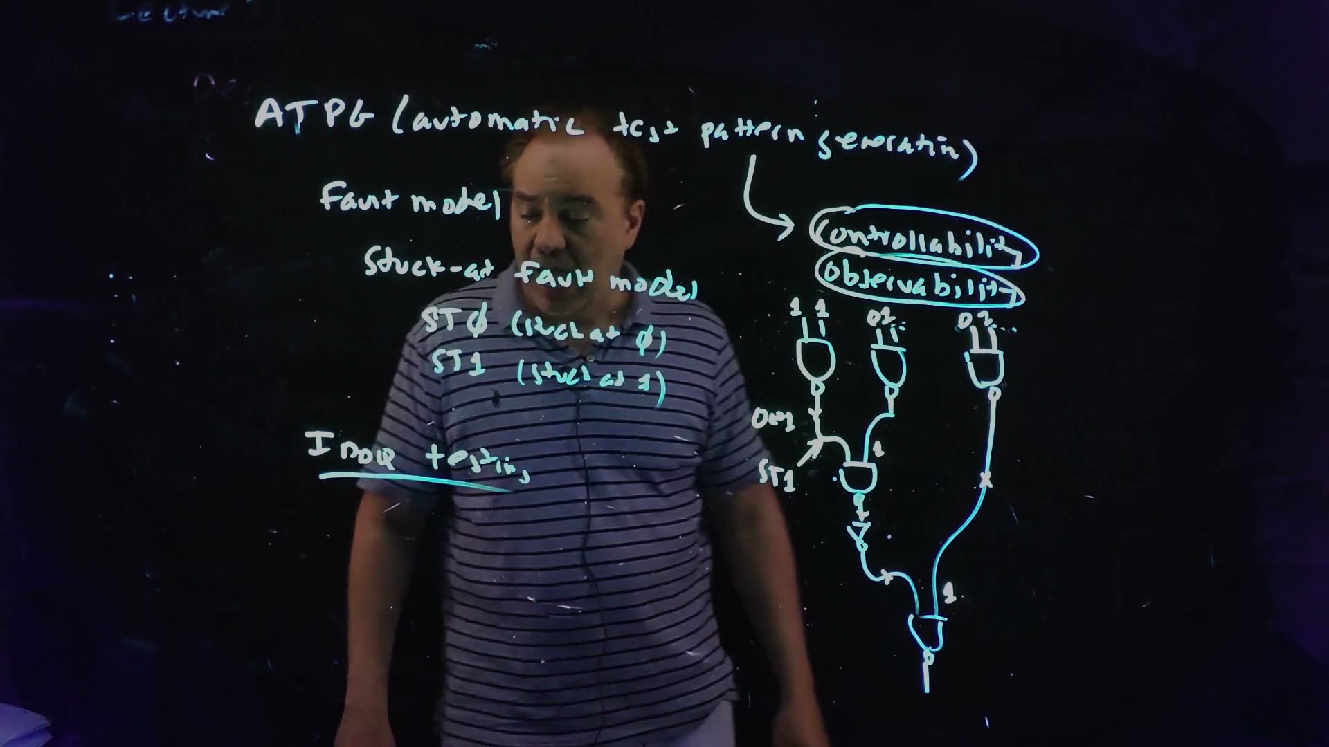
Fair copy of the board above (Lecture21 @ 44:25), mark for mark in its own layout, all in black: one cyan pen wrote the whole board, the text, the rings and the network alike (measured; the paler ATPG is the same pen). The gates are drawn as on the board, outputs down. The label beside the first gate’s output, written like 0∨1, is the good/faulty pair 0/1 on $n_1$ in the redraw; the dots after the other two input pairs are copied as written. The faint remnant of “Lecture 21” at the top left is left out.

The same pattern tests other faults (43:01–43:36). The pattern 110101 also detects, for example, $n_3$ stuck at 0 and $y$ stuck at 0: every node along the sensitized path is controlled and observed at once. The board’s × marks one more node the lecturer asks about. ATPG’s real job is a small set of patterns that together detect every fault: a design must reach a fault coverage of “usually 99.99 or something percent of the nodes” (40:22), and a node no pattern can test forces a design change.

Reconvergent fan-out

When the faulty node feeds two paths that meet again at a later gate, the difference can arrive at that gate on both inputs, and the meeting gate decides what happens added.

A worked example: X = AND(c, d) stuck at 0 (added)

1. The circuit. $X = cd$ fans out to two NANDs, $n_1 = \overline{Xa}$ and $n_2 = \overline{Xb}$Xb, which meet at an AND: $y = n_1 n_2$n1​n2​. The fault: $X$ stuck at 0.
2. Control. $X$ must be 1 in the good circuit: $c = d = 1$1. Now $X$ = 1/0.
3. Both branches. With $X$ = 0 the faulty circuit has $n_1 = n_2 = 1$ and $y = 1$1, whatever $a$ and $b$ are. The good circuit has $n_1 = \bar a$aˉ, $n_2 = \bar b$bˉ, so $y = \bar a\,\bar b$aˉbˉ.
4. When they differ. The good $y$ must be 0, so $a = 1$ or $b = 1$1. One sensitized branch is enough: with $a = 1$1, $b = 0$0, the branch through $n_1$ carries 0/1 and the other branch is a steady 1, non-controlling for the AND, so $y$ = 0/1.
5. Counting. $cd = 11$ and $ab \in \{01, 10, 11\}${01,10,11}: the patterns $abcd$ = 0111, 1011, 1111, three of the 16. Not unique.

Reconvergent fan-out added: $X = \mathrm{AND}(c, d)$AND(c,d), stuck at 0, fans out to two NANDs that reconverge at an AND. For $a = 1$1, $b = 0$0, $c = d = 1$1, the difference runs through $n_1$ (thick) while $n_2$ is a steady 1, non-controlling for the AND, so $y$ = 0/1: one sensitized branch suffices here.

Not every meeting gate is this kind. Here the AND lets either branch through, because the other branch can sit at the non-controlling 1. Two other cases appear on exams added:

• Both branches must be sensitized at once. If the faulty value arriving on a branch is the meeting gate’s controlling value, the faulty circuit’s output is pinned as soon as the fault reaches that gate on either branch. The good output differs from it only when every branch carries the good (non-controlling) value, so the pattern must open both paths together; opening just one finds nothing.
• The differences cancel. If the branches meet at an XOR and the pattern opens both, both carry the flipped value and the XOR’s output does not change. Through an XOR the pattern must open exactly one of the two branches; then the difference passes.

The safe method for any reconvergence: write the good and faulty values on both branches and evaluate the meeting gate in each circuit, or simply try the candidate pattern on both circuits.

Traps.

• A side input at its controlling value. A 0 on a NAND’s side input fixes its output at 1 and blocks the path.
• Forgetting the second branch. In reconvergent fan-out the fault reaches the meeting gate on every branch the pattern opens; evaluate them all.
• “Is the pattern unique?” without counting the don’t-cares. Count the free inputs’ choices (the lecture’s example has 9 patterns, not one).
• Losing the inversions. Each NAND and inverter on the path flips the pair: 0/1 becomes 1/0.

Check yourself In the lecture's network, find a pattern that detects n4 stuck at 1, and count how many of the 64 do.

Control: the good $n_4$ must be 0, so $n_3 = 1$1, and the second NAND needs a 0 on at least one input: $n_1 = 0$ ($ab = 11$ab=11) or $n_2 = 0$ ($cd = 11$cd=11). Of the 16 choices of $abcd$abcd, the 9 with $ab \ne 11$ and $cd \ne 11$ fail, leaving 7. Observe: $n_5$ must be 1, non-controlling for the last NAND, so $ef \ne 11$ (3 choices). For example $abcdef$ = 110000: $n_1 = 0$0, $n_3 = 1$1, $n_4$ = 0/1, $y$ = 1/0. In all, $7 \times 3 =$ 21 of the 64, which exhaustive simulation confirms.

Check yourself In the reconvergent example, find every pattern that detects X stuck at 1, and say whether it is unique.

Control: $X$ must be 0, so $cd \ne 11$ (3 choices). The faulty circuit has $X = 1$1, so $y = \bar a\,\bar b$aˉbˉ; the good one has $X = 0$0, so $n_1 = n_2 = 1$ and $y = 1$1. They differ when $a = 1$ or $b = 1$ (3 choices). So $3 \times 3 =$ 9 of the 16 patterns detect it: not unique.

Check yourself Why does fault coverage count faults, not patterns?

Because the goal is to detect every defect, and each pattern detects many faults at once (every node it controls and observes). Coverage is the fraction of all modelled faults that some pattern in the set detects; the number of patterns is the cost, which ATPG keeps small.

8. A stuck-at test through a scan chain, end to end

You need

The scan test and its bit order (Section 5). Shift the state in with SE = 1, the last flip-flop’s value first; give one capture edge with SE = 0 and the primary inputs applied; shift out with SE = 1. scan_out shows $D_n$ as soon as the capture edge has passed, then $D_{n-1}$Dn−1​, …, $D_1$ after each shift edge.

Building a stuck-at test (Section 7). Drive the faulty node to the value opposite its stuck value (control); give every side input along a path to an observed output its non-controlling value, 1 for NAND/AND and 0 for NOR/OR (observe); work back to the inputs. A value is written good/faulty.

The example circuit (Section 5). Chain scan_in → $F_1$ → $F_2$ → $F_3$ → scan_out, primary input $P$P; $G = \overline{q_1 + q_2}$q1​+q2​​, $D_1 = \overline{G\,q_3}$Gq3​​, $D_2 = \overline{G + P}$G+P​, $D_3 = q_1 q_3$q1​q3​.

The example circuit (Section 5); the cross marks $G$G, the fault site. Original figure ↑

The question. The finals ask the whole chain of reasoning at once: here is a scan chain and its logic, here is a fault; what do you shift in, in what order, what comes out of the good circuit and of the faulty one, and which bit shows the difference? This section joins Sections 4–7 on the chapter’s own circuit added. The lecture never runs a fault through a chain; the finals do.

G stuck at 0, from the fault to the bit that shows it (added)

1. The fault. $G$G, the NOR’s output, is stuck at 0 (ST0).
2. Control. The good $G$ must be 1. A NOR gives 1 only when both inputs are 0: $q_1 = q_2 = 0$0. Now $G$ = 1/0.
3. Observe. $G$ fans out to two gates, and either can carry the difference. Through the NAND to $D_1$D1​, the side input $q_3$ must be non-controlling for a NAND: $q_3 = 1$1. Through the NOR to $D_2$D2​, the side input $P$ must be non-controlling for a NOR: $P = 0$0. Choose both: $q_1q_2q_3 = 001$ and $P = 0$0.
4. Load. The first bit in ends in $F_3$F3​, so scan_in carries $q_3, q_2, q_1$ = 1, 0, 0 over three shift edges with SE = 1 (Section 5’s example).
5. Capture, SE = 0 and $P = 0$ applied by the tester. Good: $G = 1$1, $D_1 = \overline{1\cdot1} = 0$0, $D_2 = \overline{1 + 0} = 0$0, $D_3 = 0\cdot1 = 0$0: (0, 0, 0). Faulty: $G = 0$0, $D_1 = \overline{0\cdot1} = 1$1, $D_2 = \overline{0 + 0} = 1$1, $D_3 = 0$0: (1, 1, 0). In good/faulty form: $D_1$ = 0/1, $D_2$ = 0/1, $D_3$ = 0/0.
6. Read. scan_out gives $D_3, D_2, D_1$D3​,D2​,D1​: good 0, 0, 0; faulty 0, 1, 1. The first bit (on scan_out right after the capture edge) agrees; the second and third bits out reveal the fault.
7. How many patterns work. With $(q_1, q_2, q_3, P)$ free, exhaustive simulation of the two circuits finds 3 detecting patterns of the 16: 0000, 0010, 0011. All have $q_1 = q_2 = 0$ (control). 0000 and 0010 show the fault at $D_2$ ($P = 0$P=0); 0010 and 0011 at $D_1$ ($q_3 = 1$q3​=1). One observation path is enough.

The test cycle by cycle (Section 5): the last row is the faulty circuit’s scan_out, its second and third bits marked ≠. Original figure ↑

Answer the question that is asked. A paper may want the register view (the captured values $D_1, D_2, D_3$ in the flip-flops) or the scan_out sequence (the same bits in reverse, in time order). Give the one it asks for, and when in doubt both, labelled.

Traps. As Sections 5 and 7, and:

• Register values reported as the scan_out sequence, or the reverse: one is the other read backwards.
• Forgetting the primary input. $P$ is not in the chain; the tester sets it during the capture edge.
• Insisting on both paths. Here either $D_1$ or $D_2$ alone shows the fault; a pattern that opens one path is a complete answer.

Check yourself Suppose only D2 were observed (say scan_out were taken from F2). Which patterns would detect G stuck at 0 then?

The difference must reach $D_2$D2​: $q_1 = q_2 = 0$ (control) and $P = 0$ (non-controlling for the NOR); $q_3$ no longer matters. The patterns $(q_1, q_2, q_3, P)$ = 0000 and 0010.

Check yourself For G stuck at 1, how many of the 16 patterns detect it? For the load q1q2q3 = 100 with P = 0, which scanned-out bit shows it?

Control needs the good $G = 0$0, so $q_1q_2 \ne 00$00; exhaustive simulation finds 9 detecting patterns of 16. For 100, $P = 0$0: good $G = 0$ gives $(D_1, D_2, D_3) = (1, 1, 0)$(1,1,0); faulty $G = 1$ gives $(1, 0, 0)$(1,0,0). Only $D_2$ differs. scan_out reads $D_3, D_2, D_1$D3​,D2​,D1​: good 0, 1, 1; faulty 0, 0, 1. The second bit out shows the fault.

9. I_DDQ testing

You need

Static CMOS draws no current at rest. In a static CMOS gate, either the pull-up or the pull-down is off in a steady state, so no current flows from $V_{DD}$ to ground except leakage: subthreshold current through off devices and tunnelling through thin gate oxide (Chapter 4).

Ratioed logic does (Chapter 10). A pseudo-NMOS gate’s pull-up is a PFET with its gate tied to ground, always on. Whenever the pull-down is on (the output low), current flows through both, all the time.

Panel (a): a pseudo-NMOS gate, whose grounded PFET conducts whenever the output is low. Original figure ↑

The question. Before any pattern is run, one measurement already finds many bad dies. What is it, why did leakage not kill it, and what does it require of the designer?

The quiescent-current test (board, 43:57–46:57)

1. What it measures board. One of the first tests at power-on asks whether there is a short between power and ground. I_DDQ is the supply current $I_{DD}$ in the quiescent state: clocks stopped, nothing switching (the board writes “quiescent” over the Q). In a good static CMOS die it is only leakage. A large value means a defect bridging $V_{DD}$ to ground: discard the die.
2. Leakage did not end it (44:40–45:36). As subthreshold and gate leakage grew, people predicted the end of I_DDQ testing. It is still used: the measurement is compared with the leakage expected for the die, and a short shows as a clear excess.
3. The design rule board (45:36–46:57): “all sources of static power dissipation” must turn off in test. A pseudo-NMOS pull-up’s gate goes not to ground but to a test signal: 0 in normal operation (the PFET on, the gate works as before), 1 in test (the PFET off, no static current). DC-biased analog circuits likewise need a way to shut off.

Making ratioed logic I_DDQ-testable, redrawn from the board (Lecture21 @ 46:17), with the test connection from the speech (46:10–46:28). (a) A pseudo-NMOS gate: its PFET’s gate is grounded, so whenever the pull-down network conducts, a static current flows from $V_{DD}$ to ground, adding to $I_{DDQ}$IDDQ​. (b) The PFET’s gate taken to a test signal: test = 0 in normal operation (the gate works as before), test = 1 during the I_DDQ measurement (the PFET is off and the static current vanishes).

The board (Lecture21 @ 46:17)

Lecture21 @ 46:17I_DDQ testing: the quiescent current, the rule that all static power must turn off, and a pseudo-NMOS pull-up.

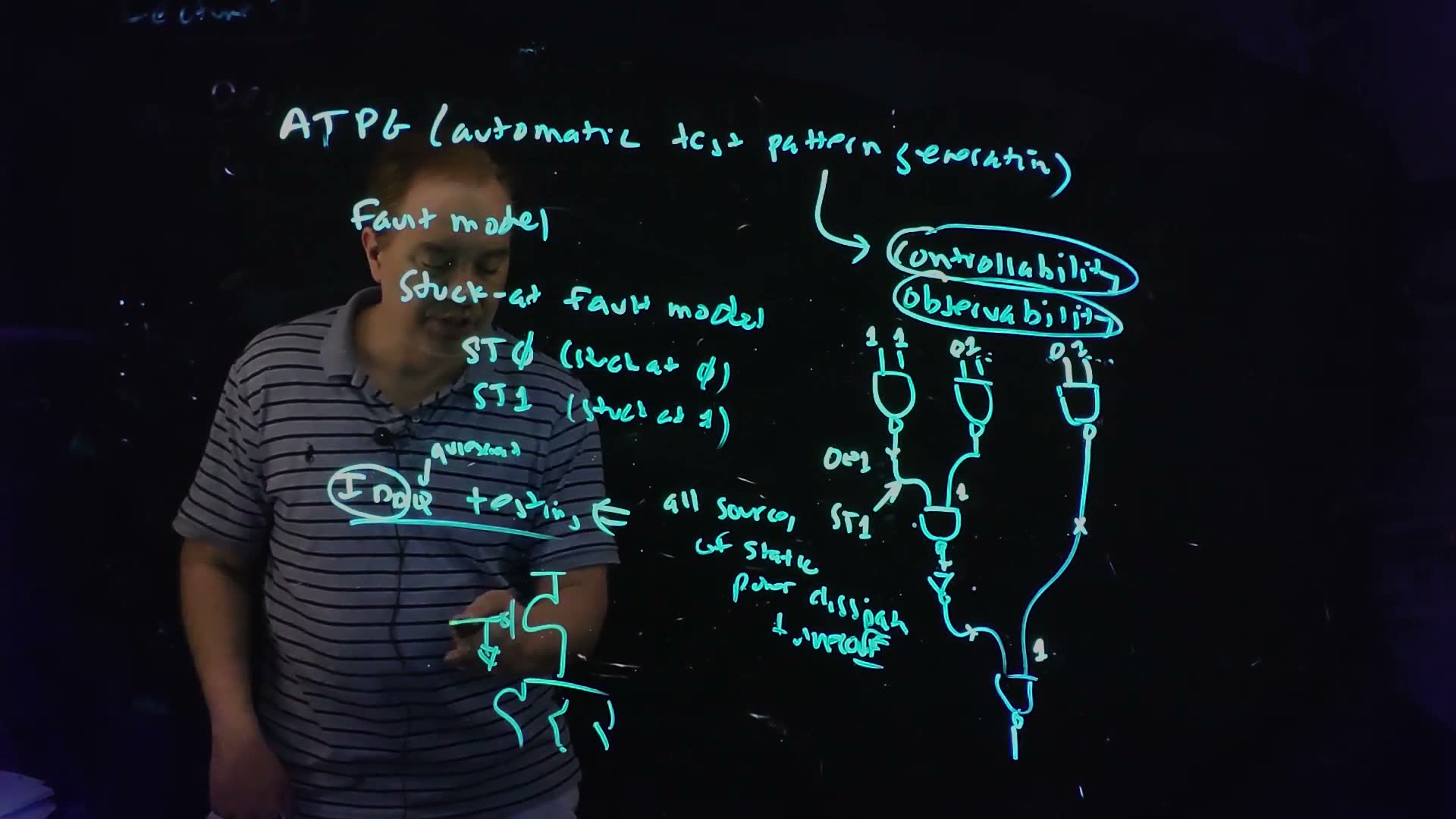
Fair copy of the board above (Lecture21 @ 46:17), mark for mark in its own layout, all in black: the same cyan pen as at 44:25, whose marks are kept unchanged. New since 44:25: the ring on I and D, “quiescent” over the Q, “⇐ all sources of static power dissipation turn OFF”, and the pull-up, its gate wire to ground, over the pull-down blob. The “test” label and its loop at the PFET’s gate, and the second underline under I_DDQ testing, appear only by 47:06, mid-erase, and were probably written after this frame, so they are left out; panel (b) of the redraw shows the connection from the speech.

Why the rule matters, in numbers added. For example, a die whose expected leakage is 20 mA at $V_{DD} = 1.0$ V:

A worked example: a short among leakage (added; values for example)

1. A 50 Ω short. It adds $I_{short} = V_{DD}/R_{short} = 1.0/50 =$ 20 mA, so I_DDQ doubles to 40 mA (2.0×): easy to see.
2. Ratioed gates left on. 500 pseudo-NMOS gates with their outputs low, each drawing 40 µA, add $500 \times 40\ \mu\text{A} =$ 20 mA: exactly what the short adds. The measurement cannot tell a good die full of ratioed gates from a shorted one.
3. With the rule. In test the ratioed gates’ PFETs are off; their 20 mA vanishes, and only the short remains to show.

$I_{short} = V_{DD}/R_{short}$ is Ohm’s law (derive); there is no other formula here.

Traps.

• “I_DDQ is a logic test.” It finds shorts whether or not they change a logic value: a weak short from a node to ground, overpowered by the gate that drives the node high, leaves every logic value right and escapes a stuck-at test, but it draws current from $V_{DD}$ whenever the node is high.
• Measuring while the chip switches. Switching current swamps any short; the measurement is quiescent by definition.
• A fixed threshold. Leakage varies from die to die and with temperature, so the limit is set against the expected leakage, with a margin.

Check yourself Why must a pseudo-NMOS pull-up be switchable on a chip that is tested by I_DDQ?

Its PFET is always on, so whenever its output is low it draws a static current from $V_{DD}$ to ground. Many such gates add up to a current that looks like a short, hiding real shorts. Taking the PFET’s gate to a test signal turns that current off during the measurement.

Check yourself With 20 mA of expected leakage at 1.0 V, what short resistance would raise I_DDQ by only 10 %? Why would that be hard to detect?

10 % of 20 mA is 2 mA, so $R_{short} = 1.0\ \text{V}/2\ \text{mA} =$ 500 Ω. The leakage itself varies from die to die by more than 10 %, so a die with this short can measure less than a good die with high leakage.

10. The bathtub curve and infant mortality

You need

Current density added. A current $I$ through a wire of width $w$ and thickness $t$ has density $J = I/(wt)$I/(wt), current per unit cross-section; narrowing the wire raises $J$ in proportion.

Electromigration, in one line added. At high current density the electrons push metal atoms along the wire, until a void opens it. Chapter 23 (Lecture 22, being written) treats it with its limits in mA/µm².

The question. Of the chips that pass every test, some still fail in customers’ hands. When do they fail, and why do the early failures happen at all?

Failures over a chip's life (board, 47:21–51:47)

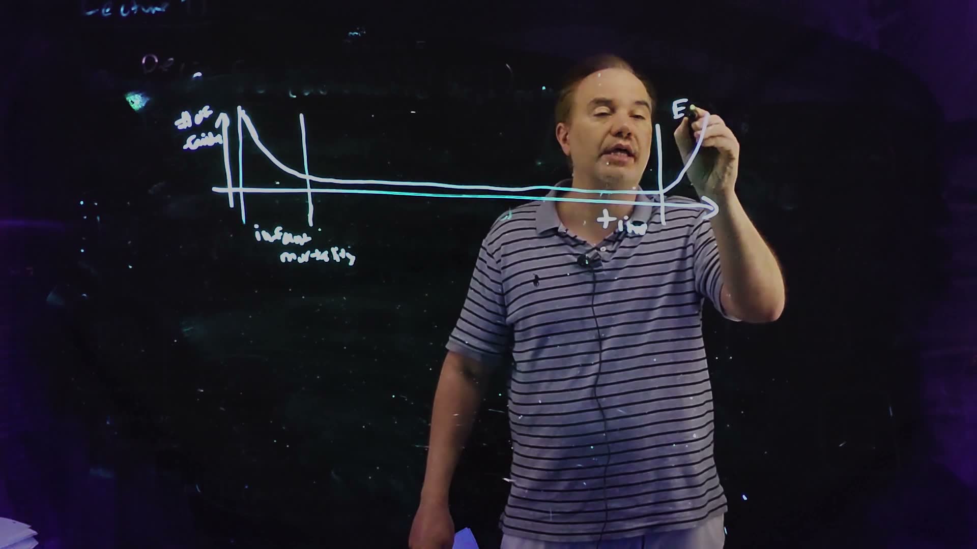
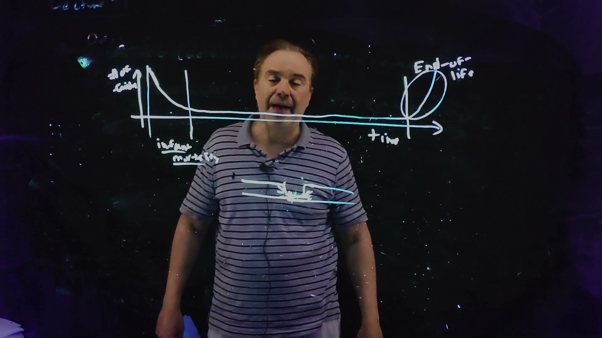
1. The bathtub curve board (49:38). Plot the number of failures against time in the field: many early, falling fast; then very few for a long time; then rising again. The shape is a bathtub’s cross-section.
2. The early region: infant mortality board. “I didn’t make up these terms, I’m sorry. This is called infant mortality” (48:22). These failures come back as warranty returns: the manufacturer’s cost.
3. The late region: end of life board (50:11). Vacuum tubes wore out routinely; solid-state devices were once thought to last forever. They do not: they wear out (Section 12), and with scaling the end of life has moved in, closer to the present (49:28–50:03).
4. Where infant mortality comes from: a latent defect board (50:30–51:47). A particle during lithography leaves a wire connected only through a narrow neck. The wire conducts, so the die passes every test: an open would have failed, a neck does not. In use, all the wire’s current crowds into the neck, and electromigration opens it after some time.

The bathtub curve, redrawn from the board (Lecture21 @ 56:35); a sketch, no values. The number of failures per unit time in the field ($N_{fail}$Nfail​) against time $t$t: region I, infant mortality (latent defects that escaped the test); region II, the useful life, with few failures; region III, the end of life (wear-out).

The board (Lecture21 @ 56:35)

Lecture21 @ 56:35The reliability board: the bathtub curve, infant mortality, the necked wire, burn-in, and wear-out with its three mechanisms.

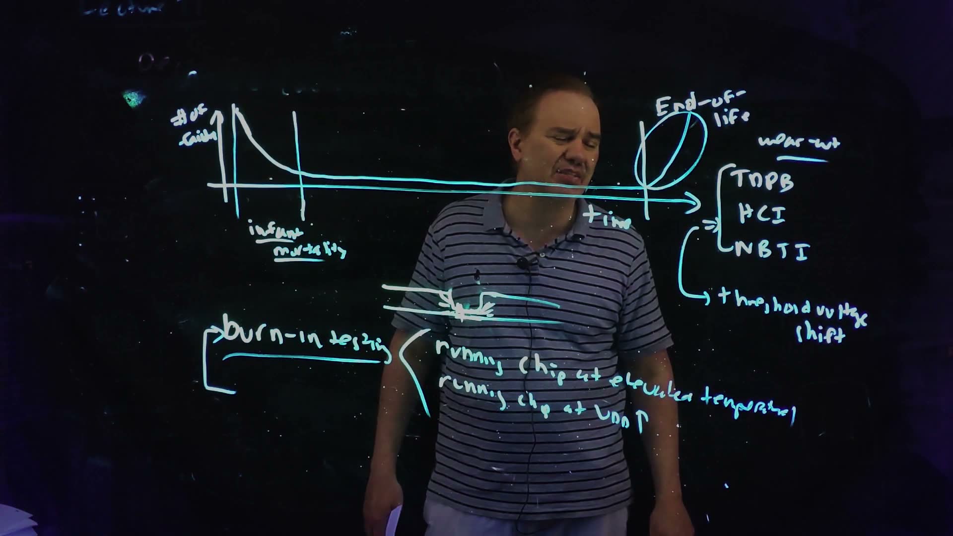
Fair copy of the board above (Lecture21 @ 56:35), mark for mark in its own layout, all in black. Two pens, white and cyan, wrote it interchangeably (each writes text as well as lines: white the curve’s fall, “infant mortality” and the three mechanisms; cyan the time axis, the dividers, the ellipse, the underlines and the brackets), so neither marks a separate layer. “failures” is set ending at the axis, where the hand crams it, and “End-of-” a little higher, clear of the ellipse. The scribble at the neck is drawn as the two converging arrows it shows.

How much worse the neck is added. The same current passes through a narrower cross-section, so the density rises by the ratio of the widths:

$$J = \frac{I}{w\,t}, \qquad \frac{J_{neck}}{J} = \frac{w}{w_{neck}} .$$

Derive it: the current and the thickness are the same on both sides of the neck; only the width changes. For example, a 1 µm wire necked to 0.25 µm carries 4 times the current density in the neck, and electromigration speeds up steeply with current density.

A latent defect, redrawn from the board (Lecture21 @ 51:47): a wire of width $w$ necked to $w_{neck}$ by a particle (drawn with $w = 4\,w_{neck}$4wneck​, the worked example’s ratio). The current $I$ (arrows) crowds into the neck, where its density is $w/w_{neck}$ times higher; electromigration opens the neck after some time in use.

Traps.

• The y axis. It is the number failing per unit time (a rate), not the cumulative number failed, which could only rise.
• “Infant mortality is a design flaw.” It is a manufacturing defect that escaped the test; the design is the same as on the good dies.

Check yourself Why does a necked wire pass the acceptance test?

It still conducts, so every logic value is right and every pattern passes; only an open would fail. The damage is in the future: the current crowded into the neck drives electromigration, which opens the wire after some time in use.

Check yourself A wire 1.2 µm wide and 0.5 µm thick carries 0.6 mA, and a particle has necked it to 0.4 µm. What is the current density away from the neck and in it?

Away from it: $J = 0.6\ \text{mA}/(1.2 \times 0.5\ \mu\text{m}^2) =$ 1.0 mA/µm². In the neck: $0.6/(0.4 \times 0.5) =$ 3.0 mA/µm², three times higher, as $w/w_{neck} = 1.2/0.4 = 3$ says.

11. Burn-in

You need

The bathtub curve (Section 10). Failures in the field are many early (infant mortality, from latent defects that escaped the test), few for a long useful life, and many again at the end of life (wear-out).

A latent defect (Section 10). A wire necked by a particle conducts, so it passes every test; in use, the current crowding into the neck drives electromigration until the wire opens.

Stress speeds failures up added. Electromigration and the other mechanisms behind latent defects run faster at higher temperature and at higher voltage (more current, higher fields).

The bathtub curve (Section 10): region I is what burn-in removes. Original figure ↑

The question. A die with a latent defect passes the acceptance test and fails weeks later. How can the manufacturer make it fail on the tester instead?

Burn-in (board, 51:55–54:11)

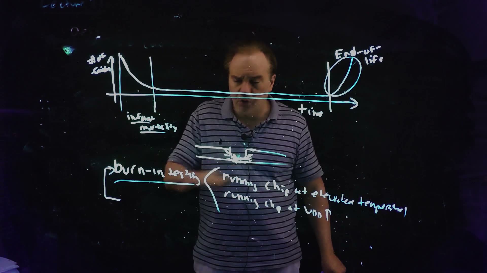
1. Stress the chip before it ships board (53:38). Burn-in testing: run the chip at an elevated temperature, “maybe” about 85 °C, and at an elevated $V_{DD}$VDD​, “maybe” about 20 % above nominal (both spoken, 51:55–52:52). “If you’re gonna fail, I’m gonna make you fail now” (52:40).
2. What it does to the bathtub added. The stress accelerates the latent-defect mechanisms, so the infant-mortality region passes in hours instead of weeks. The weak dies fail during or right after burn-in, are caught by the test that follows, and are discarded. The curve the customer sees starts on the flat bottom.
3. The rule today (53:12–54:11). Chips once had to compute correctly under burn-in conditions, which forced large design margins. Now the chip need not give the right answer under burn-in; after it returns to nominal conditions, it must work. Burn-in is meant to screen, not to damage.
4. The answer’s shape added. A question on infant mortality wants three things: one mechanism, named (a necked wire failing by electromigration); why burn-in accelerates it (temperature, voltage and so current density); and the outcome (the weak part fails on the tester and is discarded, instead of in the field).

What burn-in removes added. Burn-in spends the infant-mortality region (I, shaded) before the chip ships at $t_{ship}$tship​; the part of the curve the customer sees (thick) starts on the flat bottom.

Worked example (the spoken values, for example). A part with a 1.0 V nominal supply burns in at $1.2 \times 1.0 =$ 1.2 V; a 0.9 V part at $1.2 \times 0.9 =$ 1.08 V; both near 85 °C.

Traps.

• “Burn-in checks that the chip works hot.” It need not work during burn-in; it must work afterwards, at nominal conditions.
• Burn-in is not wear-out. It removes infant mortality; it does nothing against wear-out (Section 12), and it uses up a little of the chip’s life.

Check yourself Name one mechanism of infant mortality, and say how burn-in identifies the chips it would make fail early.

A wire necked by a particle during lithography: it conducts and passes the test, but the current crowds into the neck and electromigration opens it after some time in use. Burn-in runs the chip hot (about 85 °C) and at a raised supply (about 20 % over nominal), which accelerates electromigration, so the neck opens during burn-in; the test afterwards finds the failure and the chip is discarded instead of failing in the field.

Check yourself Why must the chip work at nominal conditions after burn-in, and what would requiring it to work during burn-in cost?

After burn-in it is a shipped product: a die damaged by the stress, or one whose defect has now opened, must be caught. Requiring correct operation at 85 °C and 20 % over-voltage would force the design to meet timing and noise margins there too: larger margins everywhere, paid for in speed or power at the conditions the chip actually runs at.

12. Wear-out: TDDB, HCI, NBTI

You need

A gate’s delay against its overdrive (Chapter 5; Chapter 21). A gate’s delay is about charge over current, $\tau \propto CV_{DD}/I_{on}$CVDD​/Ion​. For a velocity-saturated device at full overdrive, $I_{on} \propto V_{DD} - V_T$VT​, so

$$\tau \propto \frac{V_{DD}}{V_{DD} - V_T} .$$

A larger $\lvert V_T\rvert$ means less overdrive, less current and a slower gate.

The bathtub curve (Section 10): region III, the end of life, is this section’s. Original figure ↑

The question. Even a perfect die eventually fails: the bathtub rises again at the right. What wears out, how does it show, and what can a design do about it?

Wear-out (board, 54:18–56:51)

1. Three mechanisms board (56:35). TDDB, time-dependent dielectric breakdown; HCI, hot-carrier injection; NBTI, negative-bias temperature instability.
2. How they show board: “usually” as a threshold voltage shift (54:44–55:35). Charge trapped in the gate oxide over years of use raises $\lvert V_T\rvert$∣VT​∣; the overdrive falls, the devices slow, and at a fixed clock the chip eventually makes errors. (TDDB’s end point is, as its name says, the oxide breaking down; the lecture groups it with the threshold shifts added.)
3. Remedies (55:35–56:51). Delay replicas: on-chip copies of critical paths that measure how much the circuits have slowed, so the clock can be throttled down as the chip ages. Spare processors: when one core becomes too slow, a spare is switched in.

Two remedies for wear-out added, from the speech (Lecture21, 55:35–56:51). (a) A delay replica: an inverter chain that ages like the logic is timed every cycle; when its delay $t_{rep}$ no longer fits in the period $T$ with margin, the clock generator lowers $f_{clk}$ (↓). (b) A spare core (dashed) is switched in for one that has become too slow (✗).

How much slower added. Take the delay model of the Need, with $V_T$ raised by $\Delta V_T$ΔVT​:

$$\frac{\tau'}{\tau} = \frac{V_{DD} - V_T}{V_{DD} - V_T - \Delta V_T} \;\approx\; 1 + \frac{\Delta V_T}{V_{DD} - V_T} .$$

Delay change from a threshold shiftadded

$$\frac{\Delta\tau}{\tau} \approx \frac{\Delta V_T}{V_{DD} - V_T}$$

Holds when: velocity-saturated devices (Chapter 5's model: current linear in the overdrive), a small shift ΔV_T compared with the overdrive V_DD − V_T, the same V_DD

Derive it in three lines: $\tau \propto V_{DD}/(V_{DD} - V_T)$VT​); the ratio of the new delay to the old is the ratio of the overdrives, inverted; for a small shift, $1/(1 - x) \approx 1 + x$ with $x = \Delta V_T/(V_{DD} - V_T)$VT​).

A worked example: 30 mV of wear (added; values for example)

1. The values. For example, $V_{DD} = 1.0$ V, $V_T = 0.30$ V, and after years of use $\lvert V_T\rvert$ has risen by 30 mV.
2. The delay ratio. $\tau'/\tau = 0.70/0.67 =$ 1.0448: 4.48 % slower. The first-order estimate gives $0.03/0.70 =$ 4.29 %.
3. What the clock must do. A path that just met a 500 ps period (2 GHz) now needs $500 \times 1.0448 =$ 522.4 ps, so the throttled clock runs at $1/522.4\ \text{ps} =$ 1.914 GHz.
4. What a guard band buys. A design that ships with 5 % of timing margin can absorb a shift up to $\Delta V_T = (V_{DD} - V_T)(1 - 1/1.05) =$ 33.3 mV before it must slow down.

Traps.

• “Burn-in removes wear-out.” Burn-in removes infant mortality; wear-out comes at the end of a good chip’s life.
• The square law. The course’s short-channel delay is linear in the overdrive; the square law would double the estimate.
• Shifting $V_{DD}$ instead of the overdrive. The shift reduces $V_{DD} - V_T$VT​; $V_{DD}$ itself is unchanged.

Check yourself Why does a larger |V_T| slow a gate?

The on-current is proportional to the overdrive $V_{DD} - \lvert V_T\rvert$∣VT​∣, so a larger threshold leaves less overdrive and less current to charge the same load through the same voltage swing: the delay rises.

Check yourself At V_DD = 0.8 V and the same V_T = 0.30 V, what does a 30 mV shift do to the delay, and why is it worse than at 1.0 V?

$\tau'/\tau = 0.50/0.47 =$ 1.0638: 6.38 % slower (first order $0.03/0.50 = 6 \%$6%), against 4.48 % at 1.0 V. The same shift is a larger fraction of a smaller overdrive, so low-voltage designs feel wear-out more.

13. Built-in self-test: ABIST and LBIST

You need

The scan chain and its test (Sections 4–5). A mux on SE in front of every flip-flop makes them one shift register; a test shifts a state in, captures once, and shifts the result out.

SRAM arrays are not flip-flops (Chapter 19). A cache is an array of 6T cells read and written through bitlines; its cells have no mux in front and cannot be put on a scan chain.

The scan chain in its two modes (Section 4). Original figure ↑

The question. The tester is expensive and sees the chip only once. Can the chip test itself, at power-on and in the field, and what can it test that scan cannot reach?

BIST (board, 57:43–61:01)

1. BIST board, built-in self-test: circuits on the chip that test the chip, besides the external tester (57:43).
2. ABIST, array BIST board (58:15–59:08). Scan covers the flip-flops but not the memories, the L1 cache’s SRAM among them. A small state machine on the chip, the ABIST engine, writes and reads patterns through the arrays at power-on and checks the results.
3. LBIST, logic BIST board (59:08–60:02). It reuses the scan chains built for acceptance testing: at start-up, scan patterns in, clock, scan out, and check that the chip still works.
4. Where LBIST’s patterns come from board (60:02–60:30). Not from ATPG and a tester’s memory, but from an on-chip LFSR, a linear feedback shift register, which generates pseudo-random patterns. The responses are compressed into a signature and compared with the expected one. The lecture runs out of time here (“I’m gonna need more time on this”); LFSRs and signatures continue in Chapter 23 (Lecture 22, being written).

Built-in self-test added, after the board (Lecture21 @ 61:01). Top, LBIST: an LFSR supplies pseudo-random patterns to the scan chain’s scan_in; the responses from scan_out are compressed in a signature register (SIG) and compared with the expected signature. Bottom, ABIST: a small state machine writes and reads the SRAM arrays, which are not on any scan chain.

The board (Lecture21 @ 61:01)

Lecture21 @ 61:01BIST: ABIST for the arrays, LBIST reusing the scan chains, patterns from an LFSR.

Fair copy of the board above (Lecture21 @ 61:01), mark for mark in its own layout, in one white pen (black). “array” is written over the A of ABIST with a short stroke, and “logic” under the L of LBIST with an arrow. The faint, illegible remnants of erased boards at the upper right and of “Lecture 21” at the top left are left out.

Traps.

• “ABIST uses the scan chains.” It cannot: the arrays’ cells are not scannable. That is why it needs its own engine.
• “LBIST’s patterns come from ATPG.” They are pseudo-random, from the LFSR; there is no tester to supply ATPG’s patterns at start-up.

Check yourself Why can't the L1 cache be tested through the scan chains?

Its storage is an SRAM array of 6T cells, reached only through word lines and bitlines; the cells are not flip-flops with a mux in front, so they cannot be linked into a shift register. ABIST tests them instead, through the array’s own read and write circuits.

Check yourself What does LBIST reuse from acceptance testing, and what replaces the tester's two jobs, supplying patterns and checking responses?

It reuses the scan chains and the shift-capture-shift procedure. An on-chip LFSR replaces the tester’s pattern memory, and a signature register that compresses the scanned-out responses, compared with the expected signature, replaces the tester’s comparison.

On the exam

Lecture 21’s test material is examined in three of the four past finals: 50 points of stuck-at and scan questions and a 5-point short answer on burn-in, plus the problem set’s scan flip-flop. The test practice page, ft1 (being written), solves every part below in full; this chapter’s examples use other circuits, so its numbers are not those parts’ answers.

Part	Points	What it asks	Sections
FN10-3	10	a test pattern for a node stuck at 1, propagated to the output through fan-out that reconverges; is it unique?	§7 (with §6)
FN17-4a	10	the scan pattern for a node stuck at 0: the values to scan in, and in what order	§7, §8 (order §4–§5)
FN17-4b	10	the values scanned out after one capture, good and faulty	§8 (with §5)
FN19-4	20	waveforms for scan_enable, clock, scan_in and scan_out that detect a stuck-at fault, showing where it is detected	§5, §8
FN17-1e	5	one mechanism of infant mortality, and how burn-in identifies the chips it affects	§10, §11
PS5-Q3a–b	—	a static scan flip-flop from its function table; how a scan chain improves testability, and the test procedure	§4, §5

No past final tests supply resonance (§1), packaging (§2), I_DDQ testing (§9), wear-out (§12) or BIST (§13); short-answer parts can draw on any of them.

Notes for the practice page.

• Reconvergence decides FN10-3. Write the good and faulty values on both branches and evaluate the meeting gate in each circuit before choosing side values; then count the free inputs’ choices to answer “unique?”.
• The order is half of FN17-4a. Load the last flip-flop’s value first; and say that a primary input is applied during capture, not scanned.
• FN17-4b and FN19-4 read the chain. Give the register view and the scan_out sequence (reversed, the last flip-flop’s bit on scan_out right after the capture edge), and mark the first differing bit. In a waveform, change SE between clock edges, never at one.
• PS5-Q3a wants the switch-level circuit of Section 4’s cell: a transmission-gate mux on SE and $\overline{SE}$ in front of a positive-edge, static master–slave flip-flop. ft1 draws it.

Memorize.

• The scan cell: $Q^{+} = \overline{SE}\cdot D + SE\cdot SI$ at the rising edge; SE = 1 shifts, SE = 0 runs normally.
• The procedure: SE = 1, shift in ($n$n edges); SE = 0, one capture edge with the primary inputs applied (at speed for an AC test); SE = 1, shift out ($n$n edges, overlapped with the next load).
• Controlling values: 0 for NAND and AND, 1 for NOR and OR. A test: the node opposite to its stuck value; every side input on the path non-controlling.
• I_DDQ: the quiescent supply current; every static current (ratioed logic, analog bias) must turn off in test.
• Burn-in: about 85 °C and about 1.2 × $V_{DD}$VDD​; it removes infant mortality (latent defects such as a necked wire failing by electromigration), not wear-out.
• Wear-out: TDDB, HCI, NBTI → $\lvert V_T\rvert$ rises → less overdrive → slower; remedies: delay replicas with clock throttling, spare cores.
• BIST: ABIST for arrays (its own engine), LBIST through the scan chains with LFSR patterns.

Derive (with the path).

• The bit order. One shift moves every bit one place: the first bit in goes farthest (load $q_n$ first); scan_out is $F_n$‘s Q, so $D_n$ comes out first, before any shift edge.
• The hum. $f_{res} = 1/(2\pi\sqrt{LC})$ (the board’s $1/\sqrt{LC}$ is in rad/s); a burst every $N$ cycles sits at $f_{clk}/N$fclk​/N, so $N \approx f_{clk}/f_{res}$ hits it.
• A threshold shift’s delay cost. $\tau \propto V_{DD}/(V_{DD} - V_T)$VT​), so $\Delta\tau/\tau \approx \Delta V_T/(V_{DD} - V_T)$VT​).
• A neck’s current density. $J = I/(wt)$I/(wt), so $J_{neck}/J = w/w_{neck}$w/wneck​.

Method card. The playbook’s card for the stuck-at and scan family comes with ft1; until then, Sections 7 and 8 are the method.

The lecture’s boards

The boards of Lecture 21 used in this chapter (37 frames)

Lecture21 @ 01:35 Power supply network: reduce noise, R/L low, grid

Lecture21 @ 02:45 decoupling, implicit and explicit; RLC ⇒ 1/√(LC) resonances

Lecture21 @ 03:40 resonance ≈ (1/10) f_clk, low frequency

Lecture21 @ 04:42 the power-supply "hum"

Lecture21 @ 05:53 Packaging: signal interconnect / power distribution

Lecture21 @ 07:01 support and heat; plastic, ceramic (alumina), epoxy resin

Lecture21 @ 08:03 through-hole and surface-mount

Lecture21 @ 10:47 PGA, cavity up and down; through-hole pros and cons

Lecture21 @ 11:52 DIP (dual in-line)

Lecture21 @ 13:22 QFP (quad flat pack), TSOP

Lecture21 @ 14:34 BGA, ball grid array

Lecture21 @ 16:26 a bumped die and a wire-bonded die; BGA

Lecture21 @ 17:11 3-on-6 and 4-on-8 mil; solder bump, C4

Lecture21 @ 18:11 the whole packaging board

Lecture21 @ 20:33 micro C4; MCM (multichip module); TSMC InFO begun

Lecture21 @ 22:16 InFO (integrated fan-out) drawn: the final packaging board

Lecture21 @ 24:15 Design for testability: design testing

Lecture21 @ 27:46 acceptance testing; speed sorting

Lecture21 @ 28:31 functional testing, test coverage ✗

Lecture21 @ 31:35 scan-based testing, LSSD, general scan design

Lecture21 @ 32:36 the scan pair begun

Lecture21 @ 33:21 mux inputs 1 and 0, scan_enable

Lecture21 @ 33:30 the scan pair with the shift arc

Lecture21 @ 35:50 AC testing

Lecture21 @ 37:35 ATPG (automatic test pattern generation)

Lecture21 @ 39:18 fault model; stuck-at: ST0, ST1

Lecture21 @ 41:11 controllability, observability

Lecture21 @ 42:34 the NAND network with its values

Lecture21 @ 44:25 n1 stuck at 1, sensitized to the output

Lecture21 @ 46:17 I_DDQ: all static power turns off; the pull-up

Lecture21 @ 47:06 the pull-up gate to "test", mid-erase

Lecture21 @ 49:38 the bathtub curve; infant mortality

Lecture21 @ 51:47 end of life; the necked wire being drawn

Lecture21 @ 53:38 burn-in: elevated temperature and V_DD

Lecture21 @ 56:35 wear-out: TDDB, HCI, NBTI ⇒ threshold shift

Lecture21 @ 58:28 BIST: ABIST, LBIST

Lecture21 @ 61:01 LBIST ⇒ scan chain; patterns from an LFSR