FW1. Final practice: wires, repeaters and power

This page practises the final’s wire and power questions: how long a signal takes to cross a long wire or a wire tree, what widening and tapering the wire do to that time, how a clock tree’s wires and buffers add up, and how a chip’s supply is kept steady by grids and decoupling capacitance. Every past-final part on these topics is here, re-solved from the papers’ figures; the keys’ numbers are not copied, and where a key slips the page says so. The parts come in three families: Elmore wires (FN10-8, FN12-9, FN19-7), the delay from a driver to one receiver; clock-tree wires (FN17-3), the same sums on an H-tree with buffers; and power grids and decap (FN12-3, FN12-4, FN17-1b), short answers on keeping the supply still. Each family opens with a How to approach section that gives the model and the moves once, and ends with harder added variations: longer chains, setups no past paper uses, and heavier arithmetic, as the real Fall 2026 midterm was.

Every part is worked the same way: what it asks, the idea, why this formula, the solution in steps (each gives its reason first), a check by another route, the answer, and what to remember. Try each part first; open the Hint if you are stuck. The answer key’s verdict is folded at the end of each past-paper part (FN19 has no key; its parts are compared with the unofficial proposed solutions instead).

Before you start. Everything here is taught in Chapter 20 and Chapter 21, and each section below restates what it uses:

wire resistance from the sheet resistance and the number of squares, and wire capacitance per length (Chapter 20 §1);
the Elmore delay and the uniform line $\tfrac12\mathcal{R}\mathcal{C}L^2 + \mathcal{R}L\,C_{load}$ (§3, §4);
trees, side branches and the segment form (§7); widening (§8) and tapering (§10); when resistance matters (§6);
repeaters and inductance (Chapter 21 §1–§2, §6–§7); supply noise and its effect on delay (§8); grids (§9); decap, how much, where it comes from and how it is built (§10–§12).

Conventions on this page.

Units. Lengths and widths in µm, resistance in Ω, capacitance in fF. Then $1\ \Omega \times 1\ \text{fF} = 10^{-15}\ \text{s} = 10^{-3}$ ps, so a product in Ω·fF divided by 1000 is in ps ( $1\ \text{k}\Omega \times 1\ \text{fF} = 1$ ps).
The Elmore delay is the delay. As the lecture and every key do, the page quotes $T_{Elmore}$ itself as the wire’s delay, with no ln 2 factor (Chapter 20 §3).
Length. Families 1 and 2 write the length $L$ , with per-length $\mathcal{R}$ and $\mathcal{C}$ , as Chapter 20 does. Where inductance enters (FN17-3c and family 3) the length is $\ell$ , because $L$ is then an inductance, as in Chapter 21.
Pages are the papers’ printed page labels.

Symbols

Symbol	Meaning	Unit	First appears
$L$ , $W$	a wire’s length and width	µm	approach 1
$R_\square$	sheet resistance: the resistance of one square of the layer, whatever its size	Ω/□	approach 1
$L/W$	the number of squares in a wire	—	approach 1
$\mathcal{R}$ , $\mathcal{C}$	resistance and capacitance per unit length, $\mathcal{R} = R_\square/W$	Ω/µm, fF/µm	approach 1
$C_{areal}$ , $C_{fringe}$	the two parts of $\mathcal{C}$ : per area of the wire’s bottom face, and per length of its sides	fF/µm², fF/µm	approach 1
$C_{load}$	a receiver’s input capacitance, lumped at the wire’s end	fF	approach 1
$T_{Elmore}$	the Elmore delay: each capacitance times the resistance it shares with the path to the receiver	ps	approach 1
$R_k$ , $C_k$	total resistance and capacitance of path segment $k$ ( $R_1$ , $C_1$ , $R_2$ , $C_2$ for FN12-9c’s two halves)	Ω, fF	approach 1
$C_{down,k}$	all the capacitance beyond the far end of segment $k$ (side branches included)	fF	approach 1
$R_{shared}$	the resistance a capacitance’s path to the driver shares with the driver-to-receiver path	Ω	approach 1
$R_{AX}$ , $R_{AB}$ , $R_{AY}$	the wire resistance from A to node X, B, Y; likewise $R_{XB}$ , $R_{XC}$ for the branches	Ω	FN10-8
$C_{XC}$	the capacitance of the wire from X to C; likewise $C_{AX}$ , $C_{XB}$	fF	FN10-8
$C_{side}$	a side branch’s capacitance (its wire and its loads), lumped where it leaves the path	fF	FN10-8a
$\tau_{inv}$	the FO1 delay: a minimum inverter driving one copy of itself (Chapter 7)	ps	FN19-7c
$t_r$ , $t_{slew}$	an edge’s transition time (its duration); one quantity, which FN17-3c writes $t_{slew}$	ps	FN19-7c
$R_{buf}$ , $C_{buf}$	the minimum inverter’s resistance and input capacitance	kΩ, fF	Variation 2
$h$ , $k$	a repeater’s size (times the minimum inverter); the number of equal segments (the original driver counts)	—	Variation 2
$T_{min}$ , $\ell_{seg}$	the repeated wire’s best delay; its best segment length	ps, mm	Variation 2
$y$	the 200 fF tap’s distance from X along X–B (the riser counts)	µm	Variation 1
$x$ , $C_L$	the length of the 4 µm part of a two-width wire; the receiver load ( $C_{load}$ ) when it varies	µm, fF	Variation 3
$t_{buf}$ , $C_{in}$	a buffer’s delay; an inverter’s input capacitance	ps, fF	approach 2
$\tau_{silicon}$	the buffers’ share of a path’s delay, the part that moves with the supply	ps	approach 2
$C_{tree}$ , $C_B$	the whole clock tree’s capacitance (the root buffer’s load); the load at B	fF	FN17-3a
$T_{A\to B}$	the total delay from A to B: root buffer, wire and leaf buffer	ns	FN17-3a
$t_{RC}$ , $t_{LC}$	a wire’s RC (diffusion) delay $\tfrac12\mathcal{R}\mathcal{C}\ell^2$ and its LC time of flight $\sqrt{\mathcal{L}\mathcal{C}}\,\ell$	ps	approach 2
$\ell^{*}$ , $\ell_1$	the length where $t_{RC} = t_{LC}$ ; the length where $t_{LC}$ reaches the slew	mm	approach 2, FN17-3c
$F$ , $f$ , $N$ (Variation 4)	a chain’s path effort, its gain per stage, its number of stages	—	Variation 4
$\ell$	a wire’s length where inductance is in play	mm	FN17-3c
$\mathcal{L}$	inductance per unit length	nH/mm	FN17-3c
$S$	supply sensitivity of a delay, $(V_{DD}/\tau)(\partial\tau/\partial V_{DD})$	—	FN17-3b
$C_{decap}$	decoupling capacitance between the on-chip supply rails	nF	FN17-1b
$C_{sw}$	the capacitance that switches in one edge (FN17-1b’s $C_{clock}$ )	nF	FN17-1b
$L$ (family 3)	an inductance: of a supply path, or of the package’s bond wires or bumps	nH, pH	approach 3
$I$ , $\bar{I}$	a current drawn from the supply; its average	A	approach 3
$N$ , $R_1$	the number of parallel supply paths (grid straps) to a point; one path’s resistance	—, Ω	approach 3
$R_{eff}$ , $L_{eff}$	the resistance and inductance of $N$ paths in parallel	Ω, pH	approach 3
$\Delta V$ , $\Delta V_{IR}$	the supply’s droop at the circuits; its DC part, the IR drop	V	approach 3
$\varepsilon$	the allowed droop, as a fraction of $V_{DD}$	—	approach 3
$R_s$	the resistance in series with a decap	mΩ	Variation 6
$\tau$ (Variation 6)	a decap’s (or a decap cell’s) own time constant, $R_sC_{decap}$	ps	Variation 6
$C_x$ , $c_s$	explicit decap; the metal–metal decap one grid strap adds	nF	Variation 7

How to approach an Elmore wire question

Recognize it by the picture: a wire drawn as thick lines with lengths in µm, a driver at A, one or more receivers with capacitors, and a line of technology data: a width, a sheet resistance in Ω/square and a capacitance per length, sometimes as a formula in $W$ . The prompts are “calculate the Elmore delay from A to B”, “widen the wire … and recompute”, “the wire width is set to … for the first … and … for the last”, “would resistance have to be considered”, “explain why the capacitance has the functional form”.

The model. A wire has resistance along it and capacitance to ground spread along it. When the driver switches, every bit of that capacitance must be charged through the resistance between it and the driver, and the receiver’s voltage lags. The Elmore delay puts one number on the lag: add up every capacitance times the resistance its charging current shares with the path to the receiver (Chapter 20 §3, §7). Three facts turn that rule into the formulas the finals need.

A uniform segment against itself counts half. A slice $dx$ at distance $x$ from the segment’s start sees $\mathcal{R}x$ of the segment’s own resistance; on average over the segment that is half of it. So a segment with total $R$ and $C$ contributes $\tfrac12RC$ from its own capacitance (Chapter 20 §4).
Capacitance beyond a segment sees all of it. Everything past the segment’s far end, whether further along the path or on a side branch that leaves later, draws its current through the whole segment.
Off-path resistance never counts. A side branch’s capacitance counts with the resistance up to where it leaves the path; the branch’s own resistance is not crossed on the way to the receiver, so it is not in the sum. A single-pole estimate cannot represent the branch’s own shielding (Chapter 20 §7).

A path from A to B made of three segments k = 1, 2, 3 joined at dots, R2, C2 over the middle one, a dashed side stub C_side after the first, C_load at B, and a brace C_down,2 under the third segment and C_load. — The segment form (Chapter 20 §7, added): segment 2’s resistance carries half its own capacitance and all of $C_{down,2}$ ; the side branch, which leaves before it, is in $C_{down,1}$ only. Original figure ↗

Why these, and their conditions. The first is the bar-resistance law with the thickness folded into $R_\square$ , plus the areal and fringe parts of the capacitance (Chapter 20 §1, §8); memorize it. The uniform line is the segment form with one segment and the load as $C_{down}$ ; memorize it and derive the ½ (slice, sum, average). Derive the segment form in three lines: (1) every capacitance counts with the path resistance it shares with B’s path; (2) collect the terms of each path resistor $R_k$ : everything beyond its far end; (3) add half its own capacitance. All three assume grounded capacitance and a single pole. A lumped load inside a segment, or a change of width, splits that segment in two.

The moves.

Per-length values first. $\mathcal{R} = R_\square/W$ for each width; $\mathcal{C}$ from the paper’s number or its formula at that width.
Draw the path from the driver to the receiver the question names, and cut it at every branch point, every width change and every lumped load. Risers count: a branch drawn as “up 1000 µm, then 2000 µm across” is 3000 µm of wire.
Each segment’s totals, $R_k = \mathcal{R}L_k$ and $C_k = \mathcal{C}L_k$ .
Each segment’s $C_{down,k}$ , walking back from the receiver: the receiver’s load, then each segment’s capacitance and each side branch (its wire and its loads) as you pass the node it leaves from.
Sum $R_k(\tfrac12C_k + C_{down,k})$ , in Ω·fF, then divide by 1000 for ps.
Check by the other grouping: the path’s own $\tfrac12RC$ , plus the load through the whole path, plus each side branch or lumped load times the resistance it shares. The two must agree.

Decide on the way: which receiver (each has its own delay); whether a lumped load sits on the path (it counts with the resistance up to it) or on a side branch (only up to the branch point); whether $\mathcal{C}$ changes with width; whether the question wants the comparison (“explain why”) as well as the number.

Traps. Forgetting the risers. Putting a side branch’s own resistance into the sum, or leaving the side branch’s capacitance out. Dropping the ½ (that lumps all the resistance in front of all the capacitance). Squaring $L$ in the load term. Keeping 0.1 fF/µm after widening when the paper gives $\mathcal{C}(W)$ . Mixing units: Ω/µm × fF/µm × µm² is Ω·fF, a thousandth of a ps. Tapering the wrong way: narrow at the driver is the worst choice.

FN10-8: a wire tree with two receivers (20 points)

You need

The Elmore rule (Chapter 20 §3, §7). A wire is resistance with capacitance to ground spread along it; each bit of capacitance charges through the resistance between it and the driver. The Elmore delay to a receiver B adds every capacitance times the resistance it shares with the path from the driver to B. A whole side branch therefore counts at the node where it leaves the path, with the path resistance up to that node; the side branch’s own resistance does not appear.

The board’s net with two receivers (Chapter 20, Lecture19 @ 39:26): for B, the down branch’s

C_5 + C_6 + C_7

is lumped at the branch node and counts with

R_1 + R_2

. Original figure ↗

A uniform segment (Chapter 20 §4). A segment with total resistance $R$ and capacitance $C$ contributes $\tfrac12RC$ from its own capacitance (a slice at $x$ sees $\mathcal{R}x$ ; the average is half) and $R$ times everything beyond it. Summed along the path, that is the segment form, $T_{Elmore} = \sum_k R_k(\tfrac12C_k + C_{down,k})$ .

Wire values (Chapter 20 §1). $R = R_\square L/W$ , so $\mathcal{R} = R_\square/W$ ; $C = \mathcal{C}L$ . With Ω and fF, the product is in Ω·fF $= 10^{-3}$ ps.

The question (FN10-8, p13, in the paper’s words). Consider a long global wire from driver A to receivers B and C as shown below. Assume that the wire is $0.4\,\mu m$ wide and and (sic) has a resistance of 0.076 $\Omega/square$ . Its capacitance per unit length is $0.1\,fF/\mu m$ .

A wire tree. A horizontal wire runs 2000 micrometres from A to X. From X a wire rises 1000 micrometres and runs 2000 micrometres right to B, which has a 100 fF capacitor to ground. From X a wire drops 1000 micrometres and runs 3000 micrometres right to C, with a 100 fF capacitor to ground. — FN10-8’s wire tree (Final 2010, p13, redrawn): from A, 2000 µm to the branch point X; up 1000 µm and across 2000 µm to B; down 1000 µm and across 3000 µm to C; 100 fF at B and at C.

The exam’s own figure (FN10-8, p13)

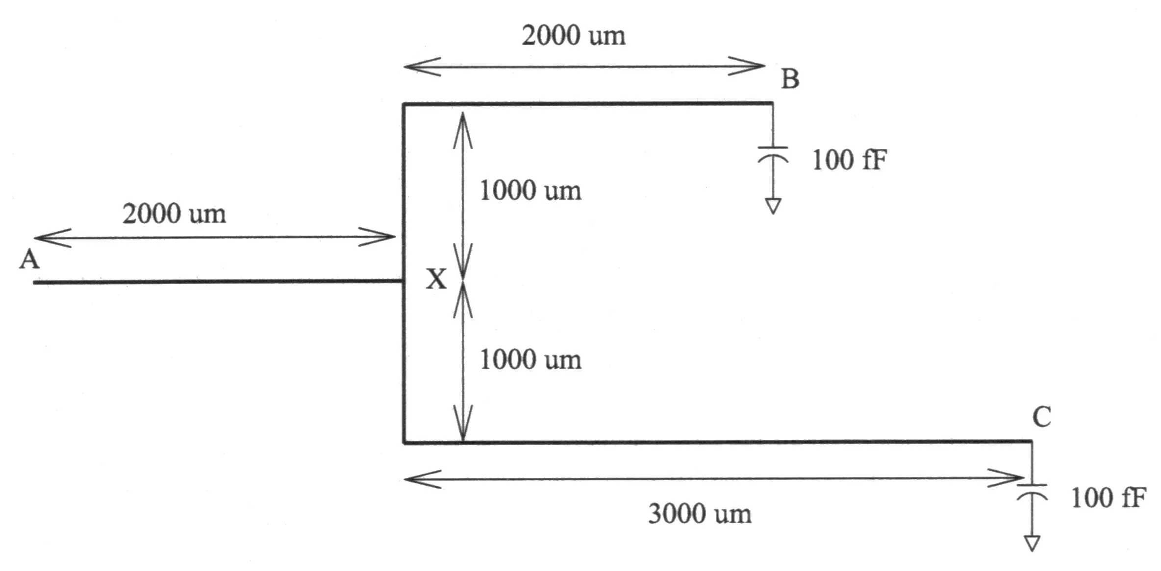
The printed wire tree: A, 2000 um to X, up 1000 um and 2000 um to B with 100fF, down 1000 um and 3000 um to C with 100fF. — FN10-8, p13 (source figure).

Reading the figure. A horizontal wire runs 2000 µm from A to the branch node X. From X, one branch rises 1000 µm and runs 2000 µm across to B; the other drops 1000 µm and runs 3000 µm across to C. So the wire from X to B is 3000 µm and from X to C 4000 µm: the risers are wire too. The width (0.4 µm) and the capacitance (0.1 fF/µm) are the same everywhere, so every segment is uniform. The receivers’ 100 fF are lumped at B and C.

Part (a): the Elmore delay from A to B (10 points)

FN10-8a, p13. Calculate the Elmore delay from A to B assuming 100 fF of loading at receivers B and C. (10 points)

FN10-8's tree: A, 2000 µm to X; up 1000 and across 2000 µm to B; down 1000 and across 3000 µm to C; 100 fF at B and C. — FN10-8’s tree (p13, redrawn): the risers are wire too. Original figure ↑

Hint

Which parts of the tree lie on the path from A to B, and what does the branch to C contribute if its resistance is not on that path?

What it asks. The time for a change at A to reach B, estimated by the Elmore delay: one number, in ps. The unknown is the sum of every capacitance in the tree times the resistance its charging current shares with the route to B. The words that decide the method are “from A to B”: the tree has two receivers and so two delays, and this part wants the one to B. That makes the wire to C a side branch: its capacitance loads the trunk, but its resistance is not on B’s path.

The idea. Everything the driver charges must pass through the trunk A–X, so the trunk’s resistance multiplies the whole tree’s capacitance beyond X, the C branch included. The branch X–B multiplies only what lies beyond it, B’s load, plus half of its own capacitance. The branch X–C’s resistance multiplies nothing that matters to B: the current into C’s wire and C’s load flows through it, but B’s voltage depends only on the voltage at X and the path from X to B. So cut B’s path into its two uniform segments, A–X and X–B, and give each its own capacitance at half weight and everything beyond it at full weight.

Why this formula. The segment form, $T_{Elmore}(A{\to}B) = \sum_{k} R_k(\tfrac12C_k + C_{down,k})$ over the path’s segments.

Where it comes from. The Elmore rule is “each capacitance times the resistance it shares with the path to B” (Chapter 20 §7). Collect the terms by path segment: segment $k$ ‘s resistance is shared by every capacitance beyond its far end, at full weight, and by its own capacitance, which sees on average half of it (the ½ of the uniform line, Chapter 20 §4).
Conditions. Every capacitance is to ground, each segment is uniform (one width, one $\mathcal{C}$ ), and the loads are lumped at the nodes. All hold here: one width everywhere, 0.1 fF/µm, the 100 fF loads at B and C.
Why not the uniform-line formula for the 5000 µm from A to B? Because it would leave out the side branch. The C branch’s 400 fF of wire and its 100 fF load are charged through A–X and slow B by doing so. (The Check of this part adds them, grouped by capacitance.)
The tempting alternatives. Putting X–C’s 760 Ω into B’s delay (it is off the path). Leaving the C branch out entirely (332.5 ps, 190 ps short). Measuring X–B as 2000 µm, without its riser.

Three path segments with a side stub after the first, C_load at B, and the brace C_down,2. — The segment form (Chapter 20 §7, added): each path segment carries half its own capacitance and all of $C_{down,k}$ . Original figure ↗

FN10-8a’s path added: for the delay to B, the thick path A–X–B carries the current, and the dashed branch X–C only loads X. Its wire $C_{XC}$ and C’s 100 fF, 500 fF in all, are lumped at X. Everything beyond X, $C_{down} = 900$ fF, charges through $R_{AX}$ .

FN10-8a

Per-length values. Because resistance comes from the number of squares, $\mathcal{R} = R_\square/W = 0.076/0.4 = 0.19\ \Omega/\mu$ m; the capacitance is given, $\mathcal{C} = 0.1$ fF/µm. (2000 µm of wire is $2000/0.4 = 5000$ squares, 380 Ω.)
The segments. Because each straight run of one width is uniform, the tree has three: A–X, 2000 µm: $R = 380\ \Omega$ , $C = 200$ fF. X–B, $1000 + 2000 = 3000$ µm: $570\ \Omega$ , $300$ fF. X–C, $1000 + 3000 = 4000$ µm: $760\ \Omega$ , $400$ fF.
What lies beyond each path segment. Because the trunk carries the current for the whole tree past X, $C_{down}$ of A–X is X–B’s 300 fF, B’s 100 fF, X–C’s 400 fF and C’s 100 fF: 900 fF. Beyond X–B there is only B’s 100 fF.
The trunk’s term. Because A–X’s own capacitance counts at half weight, $R_{AX}(\tfrac12C_{AX} + C_{down}) = 380 \times (100 + 900) = 380{,}000\ \Omega\cdot$ fF $= 380$ ps: 38 ps from its own wire, 342 ps from everything beyond X.
The branch’s term. Because X–B carries only its own capacitance and B’s load, $570 \times (150 + 100) = 142{,}500\ \Omega\cdot$ fF $= 142.5$ ps: 85.5 ps from its own wire, 57 ps from the 100 fF at B.
Add. $T_{Elmore}(A{\to}B) = 380 + 142.5 = 522.5$ ps. X–C’s 760 Ω never entered.

Check. Group the same sum the other way, by capacitance and the resistance it shares with B’s path. The path A–X–B is one uniform 5000 µm wire, $R_{AB} = 950\ \Omega$ and $C_{AB} = 500$ fF, so its own capacitance gives $\tfrac12 \times 950 \times 500 = 237.5$ ps. B’s 100 fF sees all 950 Ω: 95 ps. The side branch, $C_{XC} + 100 = 500$ fF, shares only $R_{AX} = 380\ \Omega$ : 190 ps. The total is $237.5 + 95 + 190 = 522.5$ ps, the same. A bound agrees too: the tree holds 1100 fF and no capacitance sees more than 950 Ω, so the delay cannot exceed 1045 ps. And C, at the end of the longer branch, is the later receiver: $T_{Elmore}(A{\to}C) = 380 + 760 \times (200 + 100)/1000 = 608$ ps.

Answer: $T_{Elmore}(A{\to}B) = 522.5$ ps (380 ps from the trunk A–X, 142.5 ps from the branch X–B).

Remember. Draw B’s path, cut it at the branch point, and give each path segment half its own capacitance and all of what lies beyond it, side branches included. The side branch costs its capacitance times the trunk resistance only; here that is 190 ps of the 522.5, more than a third, from a wire that does not lead to B.

Two horizontal stacked bars on a 0 to 800 ps axis. Bar (a): 237.5 (R_AB C_AB / 2), 95 (R_AB C_B), 190 (R_AX C_side, the side branch's 500 fF), total 522.5. Bar (b): the same three, then 152 (R_AY C_Y) and 76 (R_AX C_Y′, the 200 fF load on the C branch), total 750.5. — FN10-8’s delay to B, term by term added (computed from the shared-resistance split, $\mathcal{R} = 0.19\ \Omega/\mu$ m, $\mathcal{C} = 0.1$ fF/µm). (a) The path’s own wire, B’s load and the side branch lumped at X ( $C_{side} = C_{XC} + 100 = 500$ fF) give 522.5 ps. (b) The two added 200 fF loads add 152 ps (at Y, through $R_{AY}$ ) and 76 ps (the C-branch load, called Y′ here, through $R_{AX}$ ): 750.5 ps.

The answer key agrees

It writes

\tfrac12R_{A\to B}C_{A\to B} + R_{A\to B}C_{load} + R_{A\to X}(C_{X\to C} + C_{load}) = 237.5 + 95 + 190 = 522.5

ps, the grouping of the Check; re-derived with its inputs, every term matches.

Part (b): two more loads (10 points)

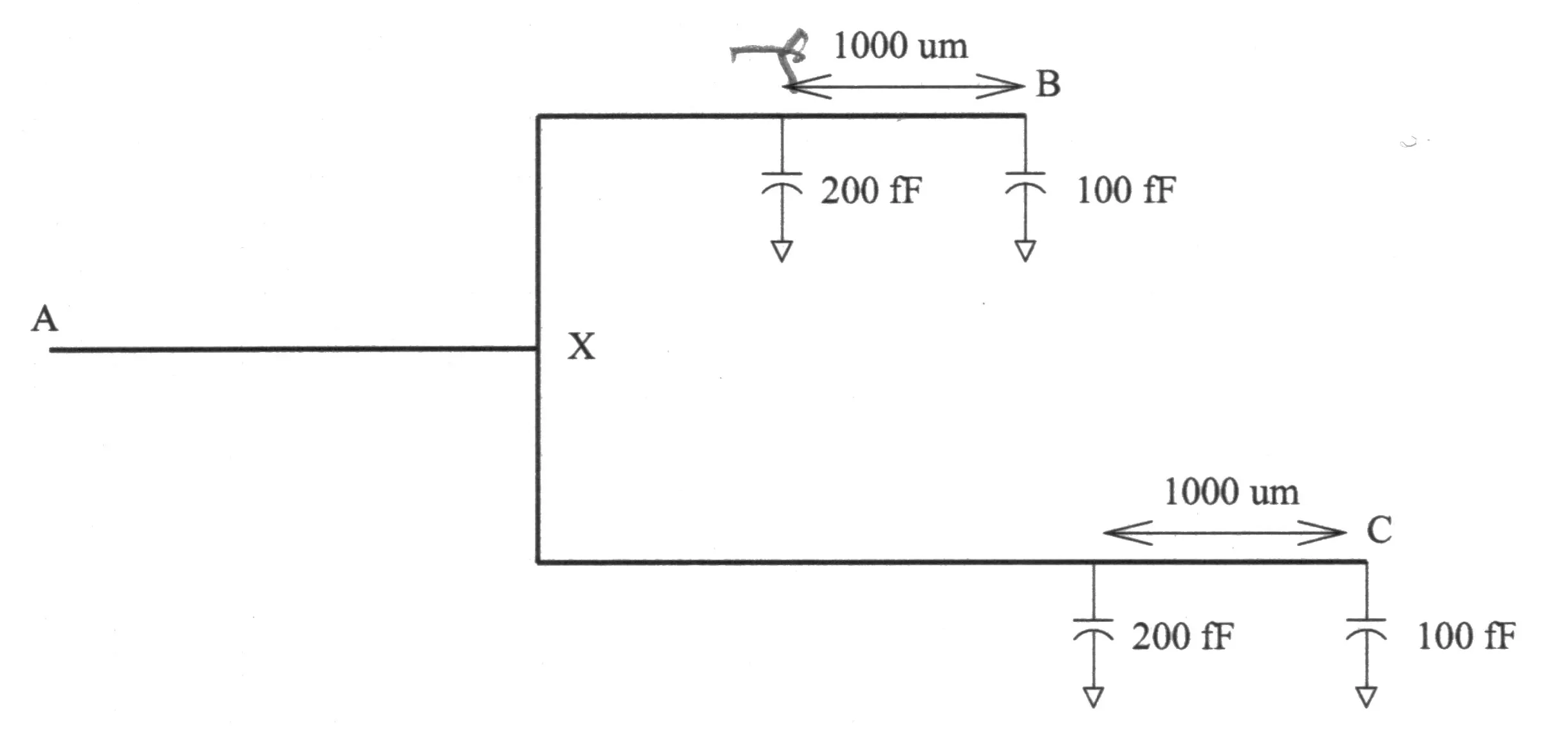
FN10-8b, p14. In addition to the receiver loading, assume that there are two additional lumped capacitance loads of 200 fF introduced $1000\,\mu m$ from each of the receivers B and C. Calculate the Elmore delay in this case from A to B. (10 points)

The same wire tree as part (a), without the long dimensions. On the run to B a 200 fF capacitor hangs 1000 micrometres before B, and B has 100 fF. On the run to C a 200 fF capacitor hangs 1000 micrometres before C, and C has 100 fF. — FN10-8b’s tree (Final 2010, p14, redrawn): part (a)‘s wires, with an extra 200 fF load 1000 µm before B and another 1000 µm before C.

The exam’s own figure (FN10-8b, p14)

The printed tree with a 200fF capacitor 1000 um before B and another 1000 um before C, 100fF at B and C; a grey hand-drawn mark at the tap before B. — FN10-8b, p14 (source figure). The grey mark at the tap before B is the key’s handwriting (its “Y”).

Hint

Each new 200 fF adds its capacitance times one resistance. Which resistance does each one share with the path to B?

What it asks. The new Elmore delay from A to B when two 200 fF loads are hung on the tree, each 1000 µm before a receiver. Everything in part (a) is still there; the unknown is what the two new loads add. The words that decide the method are “1000 µm from each of the receivers”: they place one load on B’s path and the other on the side branch to C, and the two count differently.

The idea. The Elmore sum is linear in the capacitances: adding a capacitor adds one term, the capacitor times the resistance it shares with the path to B, and changes nothing else. Call the load on the B branch Y (the key’s name; the paper does not name it). It sits on the path, 2000 µm along the B branch from X, so its current crosses the trunk and 2000 µm of that branch, and B’s voltage waits for it through all of that. The load on the C branch sits on the side branch; it shares with B’s path only the trunk, $R_{AX}$ , exactly as the rest of the side branch did in part (a).

Why this formula. A lumped capacitance $c$ adds $c \times R_{shared}(c, B)$ to $T_{Elmore}(A{\to}B)$ .

Where it comes from. It is the Elmore rule itself, applied to one capacitor (Chapter 20 §7, the shared-resistance rule). In the segment form the same thing appears as a cut: Y splits the B branch into X–Y and Y–B, and the new 200 fF enters $C_{down}$ of A–X and of X–Y, the two segments before it; the C-branch load enters $C_{down}$ of A–X only.
Conditions. As in (a): grounded, lumped loads; uniform segments; one pole. Linear superposition of the terms holds because the Elmore delay is a sum of products of fixed resistances and capacitances.
Which resistance. For Y: $R_{AY} = R_{AX} + 2000\ \mu\text{m} \times 0.19\ \Omega/\mu\text{m} = 380 + 380 = 760\ \Omega$ . For the C-branch load: $R_{AX} = 380\ \Omega$ ; the 3000 µm of C branch before it are off B’s path.
The tempting alternatives. Measuring Y from B instead of from A (using 1000 µm of resistance, 190 Ω, the distance the paper quotes). Giving the C-branch load the C branch’s resistance as well. Both come from reading the paper’s “1000 µm from each receiver” as the resistance to use; it is only the position.

The board's net with two receivers, the down branch lumped at the branch node. — The board’s net (Chapter 20, Lecture19 @ 39:26): a capacitance on the side branch counts with $R_1 + R_2$ , the shared trunk, wherever it sits on that branch. Original figure ↗

FN10-8b’s added loads added (Y is this page’s name for the tap 1000 µm before B). The 200 fF at Y charges through the resistance it shares with B’s path, $R_{AY} = 760\ \Omega$ (traced along the path). The 200 fF on the C branch shares only $R_{AX} = 380\ \Omega$ with B’s path, so it counts as if it sat at X.

FN10-8b

Start from (a). Because the sum is linear in the capacitances and nothing else changed, the delay is (a)‘s 522.5 ps plus one term for each new load.
Place the path load. Because Y is 1000 µm before B on a 3000 µm branch, it is 2000 µm from X along the branch: $R_{AY} = 380 + 0.19 \times 2000 = 760\ \Omega$ .
Its term. Because Y is on B’s path, its 200 fF counts with all of $R_{AY}$ : $760 \times 200 = 152{,}000\ \Omega\cdot$ fF $= 152$ ps.
The side-branch load. Because it hangs on the branch to C, it shares only the trunk with B’s path: $380 \times 200 = 76{,}000\ \Omega\cdot$ fF $= 76$ ps.
Add. $T_{Elmore}(A{\to}B) = 522.5 + 152 + 76 = 750.5$ ps.

Check. Redo the whole sum by the segment form, with B’s path now cut at Y into A–X, X–Y (2000 µm: 380 Ω, 200 fF) and Y–B (1000 µm: 190 Ω, 100 fF). Beyond X lie X–Y’s 200, Y’s 200, Y–B’s 100, B’s 100, the C branch’s 400 and its two loads, 200 and 100: 1300 fF, so A–X gives $380 \times (100 + 1300) = 532$ ps. Beyond Y lie Y’s 200 fF, Y–B’s 100 and B’s 100, so X–Y gives $380 \times (100 + 400) = 190$ ps. Y–B gives $190 \times (50 + 100) = 28.5$ ps. The total, $532 + 190 + 28.5 = 750.5$ ps, matches. The two equal loads cost 152 and 76 ps: exactly the ratio of their shared resistances, 760 : 380.

Answer: $T_{Elmore}(A{\to}B) = 750.5$ ps: (a)‘s 522.5 ps, plus 152 ps for the 200 fF on B’s path and 76 ps for the 200 fF on the branch to C.

Remember. A lumped load adds (its capacitance) × (the resistance it shares with the receiver’s path), and nothing else. Measure that resistance from the driver, not from the receiver. The same capacitor is worth more on the path than on a side branch, and more the farther it sits from the driver.

Two stacked bars: (a) 237.5 + 95 + 190 = 522.5 ps; (b) the same plus 152 and 76 = 750.5 ps. — FN10-8’s delay to B, term by term (computed, added): the two equal loads cost 152 and 76 ps. Original figure ↑

The answer key agrees

It adds

R_{A\to Y}(200\ \text{fF}) + R_{A\to X}(200\ \text{fF})

with

R_{A\to Y} = 0.076 \times 4000/0.4 = 760\ \Omega

and

R_{A\to X} = 380\ \Omega

522.5 + 152 + 76 = 750.5

ps. Re-derived with its inputs, every term matches; the “Y” on its figure is its own label.

FN12-9: widening and tapering a point-to-point wire (32 points)

You need

The uniform line (Chapter 20 §4). A wire of one width, length $L$ , resistance $\mathcal{R}$ and capacitance $\mathcal{C}$ per length, driving a lumped $C_{load}$ at its end, has $T_{Elmore} = \tfrac12\mathcal{R}\mathcal{C}L^2 + \mathcal{R}L\,C_{load}$ . The first term is intrinsic: the wire’s resistance against its own capacitance, each slice seeing on average half the resistance. The second is extrinsic: the whole resistance against the load. The intrinsic term grows as $L^2$ .

A driver, a uniform wire of length L with script R and script C per length, and C_load at the receiver; a slice dx at x with capacitance script-C dx sees resistance script-R x back to the driver. — The uniform line (Chapter 20, Lecture19 @ 27:59, redrawn): a slice at $x$ sees $\mathcal{R}x$ , half of $\mathcal{R}L$ on average. Original figure ↗

Capacitance against width (Chapter 20 §8). A wire’s capacitance has an areal part from its bottom face, proportional to $W$ , and a fringe part from its sides, which does not depend on $W$ : $\mathcal{C} = C_{areal}W + C_{fringe}$ . Resistance falls as $1/W$ : $\mathcal{R} = R_\square/W$ . So widening cuts the extrinsic term as $1/W$ , but in the intrinsic term only the fringe share falls; the areal share, $\tfrac12R_\square C_{areal}L^2$ , does not change with width at all.

A wire cross-section above a ground plane: vertical field lines from the bottom face (C_areal) and arcs from the sides (C_fringe); C = C_areal·W·L + C_fringe·L. — Areal and fringe capacitance (Chapter 20, Lecture19 @ 49:19, redrawn). Original figure ↗

Two segments (Chapter 20 §10). A wire made of a near segment (1) and a far segment (2) into $C_{load}$ has, by the segment form, $T = R_1(\tfrac12C_1 + C_2 + C_{load}) + R_2(\tfrac12C_2 + C_{load})$ : the near resistance multiplies everything after it; the far capacitance is seen through the near resistance as well as its own.

The question (FN12-9, p12, in the paper’s words). Consider a long point-to-point global net from driver A to receiver B as shown below. Assume that the wire is $0.4\,\mu m$ wide and has a resistance of $0.076\,\Omega/square$ . Its capacitance per unit length is given by:

0.04\ \text{fF}/\mu\text{m} + 0.15\ \text{fF}/\mu\text{m}^2 \times W

Assume the receiver at B represented a (linear) capacitance of 30 fF.

A long thick wire from A on the left, 4000 micrometres long, ending at B on the right, where a 30 fF capacitor connects to ground. — FN12-9’s wire (Final 2012, p12, redrawn): 4000 µm from the driver end A to the receiver B, which loads it with 30 fF.

The exam’s own figure (FN12-9, p12)

The printed wire: A at the left, a long line marked 4000 um, and a 30fF capacitor at B on the right. — FN12-9, p12 (source figure).

Reading the figure and the data. One wire, 4000 µm, from A to B, with B’s 30 fF at the end: a point-to-point net, no branches. The capacitance formula is Chapter 20’s areal-plus-fringe form: $C_{fringe} = 0.04$ fF/µm (the sides), $C_{areal} = 0.15$ fF/µm² (the bottom face, per µm of width). It is the reason widening is a question at all: a wider wire has less resistance but more capacitance.

Part (a): the 0.4 µm wire (10 points)

FN12-9a, p12. Calculate the Elmore delay from A to B. Hint: Remember that the Elmore delay of a distributed RC line of length L with a resistance per unit length of $\mathcal{R}$ and a capacitance per unit length of $\mathcal{C}$ is given by $\tau = \tfrac12\mathcal{R}\mathcal{C}L^2$ . (10 points)

FN12-9's wire: A, 4000 µm, B with 30 fF. — FN12-9’s wire (p12, redrawn): 4000 µm into 30 fF. Original figure ↑

Hint

The paper’s hint gives the wire against itself. What else does the wire’s resistance have to charge?

What it asks. The Elmore delay of the 4000 µm, 0.4 µm wire into B’s 30 fF, in ps. The unknowns on the way are the per-length values at this width. The paper’s own hint is the trap: it quotes only $\tfrac12\mathcal{R}\mathcal{C}L^2$ , the delay of an unloaded line, but the statement gives a 30 fF receiver, so the answer needs the load term too.

The idea. Every slice of the wire charges through the resistance between it and A: on average half the wire’s resistance, which gives the intrinsic $\tfrac12\mathcal{R}\mathcal{C}L^2$ . The receiver’s 30 fF sits at the far end and charges through all of it: the extrinsic $\mathcal{R}L\,C_{load}$ . The capacitance per length must first be read off the formula at $W = 0.4$ µm.

Why this formula. $T_{Elmore} = \tfrac12\mathcal{R}\mathcal{C}L^2 + \mathcal{R}L\,C_{load}$ .

Where it comes from. The Elmore rule (each capacitance times its resistance back to the driver) applied to a continuous line: a slice $\mathcal{C}\,dx$ at $x$ sees $\mathcal{R}x$ ; integrating from 0 to $L$ gives $\tfrac12\mathcal{R}\mathcal{C}L^2$ ; the load at the end sees $\mathcal{R}L$ (Chapter 20 §4).
Conditions. One width and one environment along the whole length (so $\mathcal{R}$ and $\mathcal{C}$ are constant), grounded capacitance, a lumped load at the end. All hold: one width, one formula, B’s 30 fF.
Why the load term belongs. The paper’s hint is the intrinsic part alone, for a line with nothing at its end. B’s 30 fF is “a (linear) capacitance”, so it is charged like any other through the whole wire.
The tempting alternatives. Stopping at the hint’s formula (152 ps). Using $\mathcal{R}\mathcal{C}L^2$ without the ½ (the wire lumped at its end). Reading $\mathcal{C}$ as 0.04 + 0.15 = 0.19 fF/µm by forgetting to multiply the areal part by $W$ .

A uniform wire of length L with script R and script C per length into C_load; a slice at x sees script-R x. — The uniform line (Chapter 20 §4): intrinsic $\tfrac12\mathcal{R}\mathcal{C}L^2$ , extrinsic $\mathcal{R}L\,C_{load}$ . Original figure ↗

FN12-9a

Capacitance at this width. Because the paper’s formula is per µm of width in its second term, $\mathcal{C} = 0.04 + 0.15 \times 0.4 = 0.04 + 0.06 = 0.10$ fF/µm: Chapter 20’s rule-of-thumb value, by design.
Resistance per length. Because a wire’s resistance is its sheet resistance times its squares, $\mathcal{R} = 0.076/0.4 = 0.19\ \Omega/\mu$ m.
The wire’s totals. Because the line is uniform, $R = 0.19 \times 4000 = 760\ \Omega$ and $C_w = 0.1 \times 4000 = 400$ fF.
Intrinsic. $\tfrac12 R\,C_w = \tfrac12 \times 760 \times 400 = 152{,}000\ \Omega\cdot$ fF $= 152$ ps.
Extrinsic. Because the 30 fF charges through the whole wire, $R\,C_{load} = 760 \times 30 = 22{,}800\ \Omega\cdot$ fF $= 22.8$ ps.
Add. $T_{Elmore} = 152 + 22.8 = 174.8$ ps.

Check. Scale from a known case. Chapter 20’s 1 mm example uses the same wire (0.4 µm at 0.076 Ω/□, 0.1 fF/µm) and has 9.5 ps of intrinsic delay; four times the length is sixteen times the intrinsic delay, $16 \times 9.5 = 152$ ps. A bound agrees: lumping all 430 fF at the far end, behind all 760 Ω, gives $760 \times 430 = 326.8$ ps, which must exceed the true sum; 174.8 ps does. The load is small next to the wire (30 fF against 400 fF), so the intrinsic part should dominate, and it does, 87 % of the total.

Answer: $T_{Elmore} = 152 + 22.8 = 174.8$ ps.

Remember. Read $\mathcal{C}$ off the width formula at the actual width first. The uniform line always has two terms when there is a receiver: the wire against itself (½, $L^2$ ) and the wire against the load (no ½, $L$ ). A paper’s hint that quotes one of them does not remove the other.

The answer key agrees

It computes

\mathcal{C} = 0.1

fF/µm and

\tfrac12(0.1)(0.076)(4000/0.4)(4000) + (0.076)(4000/0.4)(30) = 152 + 22.8 = 174.8

ps, with the load term the paper’s hint leaves out.

Part (b): widening to 4 µm (10 points)

FN12-9b, p13. Widen the wire from $0.4\,\mu m$ to $4\,\mu m$ and recompute the Elmore delay. (10 points)

Hint

When the wire is ten times wider, which of its per-length values falls tenfold, and does the other one stay put?

What it asks. The same wire, ten times wider, and its new Elmore delay. What differs from (a) is the width, so both per-length values must be recomputed: resistance falls, but the paper’s capacitance formula makes $\mathcal{C}$ rise with $W$ .

The idea. Widening lowers the resistance as $1/W$ , which helps both terms. But the wire’s bottom face grows with $W$ , so its areal capacitance grows in proportion, while its fringe capacitance stays. In the intrinsic term $\tfrac12\mathcal{R}\mathcal{C}L^2$ the areal part’s $1/W$ and $W$ cancel: that part of the delay does not move however wide the wire is. Only the fringe part and the load term fall tenfold. So expect a big cut in the 22.8 ps load term and a modest one in the 152 ps intrinsic term.

Why this formula. The uniform line again, $T_{Elmore} = \tfrac12\mathcal{R}\mathcal{C}L^2 + \mathcal{R}L\,C_{load}$ , now with $\mathcal{R} = R_\square/W$ and $\mathcal{C} = C_{areal}W + C_{fringe}$ at $W = 4$ µm.

Where it comes from. As in (a): each slice sees on average half the wire’s resistance, the load all of it (Chapter 20 §4). Putting in the width: $T(W) = \tfrac12R_\square C_{areal}L^2 + \tfrac12R_\square C_{fringe}L^2/W + R_\square L\,C_{load}/W$ (Chapter 20 §8). The first term has no $W$ .
Conditions. The wire is still uniform, now 4 µm along all 4000 µm, with the same receiver; the capacitance formula holds at 4 µm (the paper gives it for any $W$ ).
The tempting alternatives. Keeping $\mathcal{C} = 0.1$ fF/µm (that would make every term fall tenfold, 17.48 ps: the free lunch the areal capacitance forbids). Dividing (a)‘s whole answer by 10.

Delay against wire width for Chapter 20's 1 mm wire: the extrinsic part falls as 1/W, the intrinsic part levels off at a floor, the total flattens. — Widening (Chapter 20 §8, computed for its 1 mm example): the extrinsic part falls as $1/W$ , the intrinsic part only down to its areal floor. Original figure ↗

FN12-9b

Resistance per length. Because resistance goes as the number of squares, ten times the width is a tenth of the squares: $\mathcal{R} = 0.076/4 = 0.019\ \Omega/\mu$ m, and $R = 0.019 \times 4000 = 76\ \Omega$ .
Capacitance per length. Because the areal term grows with the width, $\mathcal{C} = 0.04 + 0.15 \times 4 = 0.64$ fF/µm, and $C_w = 0.64 \times 4000 = 2560$ fF: 6.4 times (a)‘s 400 fF.
Intrinsic. $\tfrac12 R\,C_w = \tfrac12 \times 76 \times 2560 = 97{,}280\ \Omega\cdot$ fF $= 97.28$ ps (from 152).
Extrinsic. Because the load has not changed and the resistance has fallen tenfold, $76 \times 30 = 2280\ \Omega\cdot$ fF $= 2.28$ ps (from 22.8).
Add. $T_{Elmore} = 97.28 + 2.28 = 99.56$ ps.

Check. Use the width law instead of the totals. For this wire, $T(W) = 91.2\ \text{ps} + 33.44\ \text{ps}\cdot\mu\text{m}/W$ : the 91.2 ps is $\tfrac12 R_\square C_{areal} L^2 = \tfrac12 \times 0.076 \times 0.15 \times 4000^2$ Ω·fF, the areal part that no width changes, and the 33.44 is the fringe part (24.32) plus the load part (9.12). At $W = 0.4$ it gives $91.2 + 83.6 = 174.8$ ps, part (a); at $W = 4$ , $91.2 + 8.36 = 99.56$ ps. The load term fell exactly tenfold (22.8 → 2.28), as $1/W$ says it must. Ten times the width bought only a 43 % cut, because most of (a)‘s delay was areal.

FN12-9’s 4000 µm wire into 30 fF, delay against width added (computed from $T(W) = 91.2\ \text{ps} + 33.44\ \text{ps}\cdot\mu\text{m}/W$ ). Widening from 0.4 µm (a) to 4 µm (b) cuts the delay from 174.8 to 99.56 ps, but no uniform width beats the areal floor of 91.2 ps. The tapered wire of part (c), which has no single width, reaches 82.46 ps (star, at the right margin).

Answer: $T_{Elmore} = 97.28 + 2.28 = 99.56$ ps, from 174.8 ps; the wire’s capacitance rises from 400 to 2560 fF.

Remember. Widening divides the resistance by the width ratio but multiplies the areal capacitance by it, so the intrinsic delay falls only to a floor, $\tfrac12R_\square C_{areal}L^2$ ; the load term always falls as $1/W$ . The bill is a wire with 6.4 times the capacitance, which the driver has to charge and which costs power: the reason the next part tapers instead.

The answer key agrees

It computes

\mathcal{C} = 0.64

fF/µm and

97.3 + 2.28 = 99.6

ps, which is 99.56 ps rounded (its 97.3 is 97.28).

Part (c): tapering (12 points)

FN12-9c, p13. Now assume that the wire width is set to $4\,\mu m$ for the first $2000\,\mu m$ and $0.4\,\mu m$ for the last $2000\,\mu m$ . Compare with your result in (b) and explain why such wire “tapering” might be advantageous. (12 points)

A wire from A to B in two halves of 2000 micrometres: the left half thick, W = 4 µm, R1 = 38 ohm, C1 = 1280 fF; the right half thin, W = 0.4 µm, R2 = 380 ohm, C2 = 200 fF. B has a 30 fF capacitor to ground. — FN12-9c’s tapered wire added: the half nearer the driver 4 µm wide, the far half 0.4 µm, each 2000 µm, into B’s 30 fF. Widths not to scale.

Hint

In the Elmore sum, whose capacitance does the near half’s resistance multiply, and whose resistance does the far half’s capacitance see?

What it asks. Three things: the Elmore delay of a wire that is 4 µm wide for its first 2000 µm (the driver’s half) and 0.4 µm for its last 2000 µm; a comparison with (b)‘s uniformly wide wire; and the reason the taper helps. What differs from (b) is that the wire is no longer uniform, so the single uniform-line formula no longer applies: it is two uniform segments in series. “Explain why” is worth points in its own right.

The idea. In the Elmore sum, resistance near the driver is expensive, because every capacitance after it charges through it; capacitance near the receiver is expensive, because it charges through every resistance before it. So the near half should have low resistance (wide), and the far half low capacitance (narrow). The far half’s resistance multiplies only its own capacitance and the 30 fF load, both small, so its being narrow costs little. The taper keeps the wide wire where width pays and drops it where it doesn’t.

Why this formula. The segment form with two segments: $T = R_1(\tfrac12C_1 + C_2 + C_{load}) + R_2(\tfrac12C_2 + C_{load})$ , segment 1 near the driver.

Where it comes from. The Elmore rule regrouped by segment (Chapter 20 §7, §10): segment 1’s resistance carries half its own capacitance and all of segment 2 and the load; segment 2’s carries half its own and the load.
Conditions. Each half is uniform (one width, so one $\mathcal{R}$ and one $\mathcal{C}$ ), capacitance grounded, the load lumped at B. The capacitance formula applies to each half at its own width.
Why not the uniform-line formula. With two widths there is no single $\mathcal{R}$ and $\mathcal{C}$ ; averaging them would hide exactly the effect the question is about (the order of the halves).
The tempting alternatives. Adding the two halves’ separate uniform-line delays (that drops the cross term $R_1C_2$ : the far half’s capacitance does charge through the near half). Using the near half’s $\mathcal{C}$ for the far half. Tapering the other way round (561.26 ps, the worst of all).

Top: a driver, a wire that steps from wide to narrow toward the receiver, with a check mark. Bottom: the opposite taper, narrow at the driver and wide at the receiver, with a cross. — Tapering (Chapter 20, Lecture19 @ 55:29, redrawn): wide near the driver, narrow near the receiver (top) beats the opposite (bottom). Original figure ↗

FN12-9c

The near half (4 µm, 2000 µm). Because the width is (b)‘s, $\mathcal{R} = 0.019\ \Omega/\mu$ m and $\mathcal{C} = 0.64$ fF/µm: $R_1 = 38\ \Omega$ , $C_1 = 1280$ fF.
The far half (0.4 µm, 2000 µm). Because the width is (a)‘s, $\mathcal{R} = 0.19\ \Omega/\mu$ m and $\mathcal{C} = 0.10$ fF/µm: $R_2 = 380\ \Omega$ , $C_2 = 200$ fF.
The near half’s term. Because $R_1$ carries half its own capacitance, the whole far half and the load, $38 \times (640 + 200 + 30) = 38 \times 870 = 33{,}060\ \Omega\cdot$ fF $= 33.06$ ps.
The far half’s term. Because $R_2$ carries only half its own capacitance and the load, $380 \times (100 + 30) = 49{,}400\ \Omega\cdot$ fF $= 49.4$ ps.
Add. $T_{Elmore} = 33.06 + 49.4 = 82.46$ ps.
Compare with (b). Because (b) is the same length wide all the way, the taper is $99.56 - 82.46 = 17.1$ ps faster (17.2 %), and its wire has $1280 + 200 = 1480$ fF of capacitance against (b)‘s 2560 fF (42 % less) on 55 % of (b)‘s metal area.
Why it helps, term by term. Because (b) is the same two halves, both 4 µm, write it in the same four terms: $\tfrac12R_1C_1 = 24.32$ , $R_1C_2 = 38 \times 1280 = 48.64$ , $\tfrac12R_2C_2 = 24.32$ , $(R_1{+}R_2)C_{load} = 76 \times 30 = 2.28$ ps. Narrowing the far half changes the last three. Its capacitance falls from 1280 to 200 fF, so the term where the near resistance charges it falls from 48.64 to 7.6 ps: 41.04 ps saved. Its resistance rises tenfold, but that resistance multiplies only its own (now small) capacitance and the 30 fF load: its own term rises from 24.32 to 38 ps (13.68 ps) and the load term from 2.28 to 12.54 ps (10.26 ps). Net, $41.04 - 13.68 - 10.26 = 17.1$ ps saved. The near half keeps (b)‘s low resistance where it multiplies everything.

The width law (computed, added): no uniform width goes below 91.2 ps; the taper does. Original figure ↑

Check. A bound from (b)‘s width law: a uniform wire of any width has at least the areal floor, 91.2 ps. The taper, at 82.46 ps, is below every uniform width, so it is not just a cheaper (b): no amount of uniform widening can match it. With the same metal (a uniform 2.2 µm wire, the taper’s average width) the delay is $91.2 + 33.44/2.2 = 106.4$ ps. And the order matters, not the metal: the same two halves the other way round (narrow at the driver) give 561.26 ps.

Three stacked bars on a 0 to 200 ps axis. (a): grey 152 and white 22.8, total 174.8, wire 400 fF. (b): grey 97.28 and a thin white 2.28, total 99.56, wire 2560 fF. (c): grey 24.32 (R1 C1 / 2), 7.6 (R1 C2), 38 (R2 C2 / 2), and white 12.54 ((R1 + R2) C_load), total 82.46, wire 1480 fF. — FN12-9’s three wires, term by term added (computed from their Elmore sums). Grey: the wire charging its own capacitance; white: the 30 fF load. Totals 174.8 ps (a), 99.56 ps (b) and 82.46 ps (c); under each bar, its wire capacitance: 400, 2560 and 1480 fF.

Answer: $T_{Elmore} = 33.06 + 49.4 = 82.46$ ps, 17.1 ps faster than (b)‘s 99.56 ps, with 1480 fF of wire capacitance instead of 2560 fF. Tapering helps because the Elmore sum weights the resistance near the driver by all the capacitance after it, and the capacitance near the receiver by all the resistance before it: a wide (low-resistance) near half and a narrow (low-capacitance) far half lower both weights, so the wire is faster, lighter for the driver to charge, and uses less routing.

Remember. A wire of two widths is two segments: the near one carries everything after it. Taper wide → narrow from the driver. It wins when the load is small next to the wire’s own capacitance (30 fF against more than 1000 fF here); with a large load the far half’s resistance would multiply that load and the gain shrinks or reverses (Variation 3: the 50/50 taper ties the uniform 4 µm wire at 80 fF; Chapter 20 §10).

The answer key agrees

Its total, 82.44 ps, is 82.46 ps with the first term rounded to 24.3 (it is 24.32). Its first line writes the sheet resistance as 0.046 Ω/□, a slip it does not carry into the number (with 0.046 that term would be 14.72 ps). It gives no comparison or explanation, which the part asks for and grades.

FN19-7: a wire tree whose capacitance depends on its width (36 points)

You need

Wire values with width (Chapter 20 §1, §8). A wire of width $W$ on a layer of sheet resistance $R_\square$ has $\mathcal{R} = R_\square/W$ per unit length. Its capacitance per length has an areal part from its bottom face, proportional to $W$ , and a fringe part from its sides, which does not depend on $W$ : $\mathcal{C} = C_{areal}W + C_{fringe}$ . Widening lowers $\mathcal{R}$ and raises $\mathcal{C}$ .

The Elmore rule on a tree (Chapter 20 §3, §7). The delay to a receiver B adds every capacitance times the resistance it shares with the path from the driver to B. By path segment, $T_{Elmore}(A{\to}B) = \sum_k R_k(\tfrac12C_k + C_{down,k})$ : each path segment carries half its own capacitance and everything beyond its far end, side branches included; a side branch’s own resistance never enters.

When resistance matters (Chapter 20 §6). The receiver sees the driver’s edge through one pole $\tau = T_{Elmore}$ . If $T_{Elmore}$ is much shorter than the edge’s transition time, the wire is just a capacitance; if it is comparable or longer, its resistance must be in the model. Edges take a few gate delays.

The question (FN19-7, p15, in the paper’s words). Consider a long global wire from driver A to receivers B and C as shown below. Assume that the wire is 0.4 mm (sic) wide and has a resistance of 0.076 Ω/square. Its capacitance per unit length is given by:

0.04\ \text{fF}/\mu\text{m} + 0.15\ \text{fF}/\mu\text{m}^2 \times W

Assume that each receiver has a load of 100 fF.

A wire tree. 2000 micrometres from A to X; from X up 1000 and across 2000 micrometres to B; from X down 1000 and across 3000 micrometres to C. — FN19-7’s wire tree (Final 2019, p15, redrawn): the same geometry as FN10-8, with no capacitors drawn; the statement gives each receiver a 100 fF load.

The exam’s own figure (FN19-7, p15)

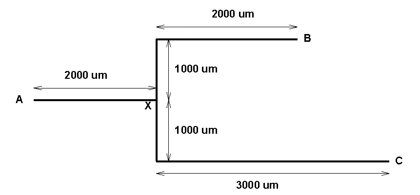
The printed branched wire: A, 2000 um to X; up 1000 um and 2000 um to B; down 1000 um and 3000 um to C; no capacitors drawn. — FN19-7, p15 (source figure). The receivers’ 100 fF are in the text, not on the drawing.

Reading the figure and the data. The tree is FN10-8’s, to the micron: 2000 µm from A to the branch point X, then 3000 µm from X to B (a 1000 µm riser and a 2000 µm run) and 4000 µm from X to C (1000 µm down, 3000 µm across). The capacitance law is FN12-9’s: $C_{fringe} = 0.04$ fF/µm and $C_{areal} = 0.15$ fF/µm². The paper prints the width as “0.4 mm” here and “0.4 µm” in part (d) (p17); read it as 0.4 µm, because part (d) widens the wire “from 0.4 µm”, and a 400 µm wide wire would make part (d) a narrowing. It also prints the Ω of the sheet resistance as a capital O. Each receiver’s 100 fF sits at B and at C.

Part (a): why the capacitance has this form (8 points)

FN19-7a, p15. Explain why the capacitance has the functional form specified above. (8 points)

FN19-7's tree: A, 2000 µm to X; up 1000 and across 2000 µm to B; down 1000 and across 3000 µm to C. — FN19-7’s tree (p15, redrawn); each receiver has 100 fF. Original figure ↑

Hint

Picture the wire’s cross-section over the layer below it. Which of its surfaces grows when the wire is made wider?

What it asks. A physical explanation, not a number: why the capacitance per unit length is a constant plus a term proportional to the width. The word that decides the answer is “functional form”: the reader must say what each of the two terms is and why one depends on $W$ and the other does not. Numbers help the explanation, but the points are for the physics.

The idea. A wire’s capacitance is the charge it holds per volt against the conductors around it: the substrate or the metal layer below (and above), and its neighbours. The electric field lines leave the wire’s surface and end on those conductors. Lines from the bottom face run almost straight down, like a parallel-plate capacitor, and that face is $W$ wide, so this part grows in proportion to $W$ . Lines from the sides curve out and down to the same plane; the sides are as tall as the metal is thick, whatever the width, so that part does not change when the wire is widened. Each part is per unit length, because every slice of the wire looks the same.

Why this formula. $\mathcal{C} = C_{areal}W + C_{fringe}$ , Chapter 20’s form.

Where it comes from. The parallel-plate law (background from circuits, added): two plates of area $A$ a distance $d$ apart have $C = \varepsilon A/d$ . For one micron of wire the bottom face has area $W \times 1\ \mu$ m, so the areal part per length is $(\varepsilon/d)\,W$ : the coefficient $C_{areal} = \varepsilon/d$ is a capacitance per unit area, in fF/µm². The side (fringing) field is not a plate, but its geometry is fixed by the metal’s thickness and the spacing, not by $W$ , so it is a constant per unit length, $C_{fringe}$ in fF/µm (Chapter 20 §8, the board at 49:19).
Conditions. The width is large enough that the sides do not interact with each other, and the surroundings (the plane below, the neighbours) stay the same as the wire widens. Both are the assumptions behind the paper’s linear law; for a very narrow wire, or one with close neighbours, the fringe part would change too.
The tempting alternative. Saying “capacitance is proportional to area” and stopping. That predicts $\mathcal{C} \to 0$ as $W \to 0$ ; the constant 0.04 fF/µm says a wire of almost no width still has its sides.

The two parts of the capacitance (Chapter 20, Lecture19 @ 49:19, redrawn): the bottom face’s straight lines grow with

W

; the sides’ fringing lines do not. Original figure ↗

A straight line of capacitance per length against width, from 0.04 fF/µm at zero width (labelled C_fringe = 0.04) to 1.54 at 10 micrometres. A dot marks 0.10 at 0.4 µm. A slope triangle with run 2 and rise 0.3 is labelled C_areal = 0.15 fF/µm². — FN19-7’s capacitance per unit length against width added (computed from $\mathcal{C} = 0.04 + 0.15W$ fF/µm): the intercept is the fringe part, the slope the areal part. At the minimum 0.4 µm it is 0.10 fF/µm; at 10 µm, 1.54.

FN19-7a

Name the two terms. Because the formula has a constant and a term in $W$ , match them to the two kinds of field line: $0.15\ \text{fF}/\mu\text{m}^2 \times W$ is the areal (parallel-plate) capacitance of the bottom face, and $0.04$ fF/µm is the fringe capacitance of the sides.
Why the areal term grows with $W$ . Because the bottom face is $W$ wide, one micron of wire has $W$ square microns of plate facing the layer below, at 0.15 fF per square micron.
Why the fringe term does not. Because the sides are the metal’s thickness tall and the field curving off them reaches the same plane, their contribution is fixed per unit length; widening the wire moves the sides apart but does not change them.
The numbers at this width. Because the paper’s width is 0.4 µm, $\mathcal{C} = 0.15 \times 0.4 + 0.04 = 0.06 + 0.04 = 0.10$ fF/µm: 60 % areal and 40 % fringe. It is Chapter 20’s rule-of-thumb 0.1 fF/µm, which is why the course quotes that value for a minimum-width wire.
What it means for widening. Because only the areal part grows, a wire 25 times wider (10 µm, part (d)) has $0.15 \times 10 + 0.04 = 1.54$ fF/µm, 15.4 times more, and the fringe is only 2.6 % of it. Resistance falls 25 times, capacitance rises 15.4 times: that trade is what part (d) measures.

Check. Ask whether 0.15 fF/µm² is a sensible plate. With silicon dioxide between the plates ( $k = 3.9$ , $\varepsilon = 3.9\varepsilon_0$ , and $\varepsilon_0 = 8.854 \times 10^{-3}$ fF/µm), a plate capacitance of 0.15 fF/µm² needs $d = \varepsilon/C_{areal} = 0.23$ µm: a dielectric a few tenths of a micron thick, the size of the layers between metal levels. (This is an order-of-magnitude check, added; the real areal part also counts the layer above.) The units agree as well: fF/µm² times µm is fF/µm, the same unit as the constant.

Answer: the capacitance per length is the sum of an areal (parallel-plate) part from the wire’s bottom face, which is proportional to its width, $0.15\ \text{fF}/\mu\text{m}^2 \times W$ , and a fringe part from the field lines that curve off its sides, which depends on the metal’s thickness and the spacing but not on the width, $0.04$ fF/µm. At 0.4 µm they give 0.06 + 0.04 = 0.10 fF/µm.

Remember. Area term ∝ $W$ (plate), fringe term constant (sides). Read $\mathcal{C}$ off the formula at the actual width before any delay sum, and expect widening to raise the capacitance less than it lowers the resistance.

The answer key agrees

FN19 has no official key. The unofficial proposed solution gives the same two terms: a width-independent fringing (sidewall) part and a plate part proportional to the width, with the units checked.

Part (b): the Elmore delay from A to B (10 points)

FN19-7b, p16. Calculate the Elmore delay from A to B. (10 points)

Hint

What does the capacitance law give at 0.4 µm, and which segments lie on the path from A to B?

What it asks. The Elmore delay from A to receiver B through the tree, in ps. What is new against FN10-8a is only the capacitance, now given by a width law; at the paper’s width it must first be evaluated. “From A to B” decides the path: A–X–B, with the branch to C a side branch.

The idea. The one difference from FN10-8a is the capacitance law, and at 0.4 µm it gives FN10-8’s 0.1 fF/µm; the sheet resistance and width are FN10-8’s too. So every segment has FN10-8’s resistance and capacitance, and the method is the same: the trunk A–X carries the whole tree beyond X, the side branch to C included; the branch X–B carries only B’s load; X–C’s resistance is off B’s path.

Why this formula. The segment form, $T_{Elmore}(A{\to}B) = \sum_k R_k(\tfrac12C_k + C_{down,k})$ over A–X and X–B, is the Elmore rule (each capacitance times the resistance it shares with B’s path) regrouped by segment: a segment’s resistance carries everything beyond it at full weight and its own capacitance at half (Chapter 20 §7). It needs grounded capacitance, uniform segments and lumped loads, all true here; one uniform line from A to B would leave out the branch to C, whose 500 fF charges through the trunk. The tempting alternatives: 0.19 fF/µm (adding 0.04 and 0.15 without the $W$ ), X–C’s resistance in B’s delay, and X–B measured without its riser.

The tree with the path A–X–B thick: A–X 380 ohm, 200 fF; X–B 570 ohm, 300 fF; the dashed branch X–C 760 ohm, 400 fF, lumped at X with C's load as 500 fF; C_down = 900 fF beyond X. — FN10-8a’s path, which is this tree at 0.4 µm added: the trunk carries the 900 fF beyond X. Original figure ↑

FN19-7b

Per-length values at 0.4 µm. Because the capacitance law depends on the width, evaluate it first: $\mathcal{C} = 0.04 + 0.15 \times 0.4 = 0.10$ fF/µm. Because resistance is sheet resistance times squares, $\mathcal{R} = 0.076/0.4 = 0.19\ \Omega/\mu$ m.
The segments. Because each straight run of one width is uniform: A–X, 2000 µm, $380\ \Omega$ , $200$ fF; X–B, 3000 µm, $570\ \Omega$ , $300$ fF; X–C, 4000 µm, $760\ \Omega$ , $400$ fF.
What lies beyond. Because the trunk feeds the whole tree past X, $C_{down}$ of A–X is $300 + 100 + 400 + 100 = 900$ fF; beyond X–B there is only B’s 100 fF.
The trunk’s term. $380 \times (\tfrac12 \times 200 + 900) = 380 \times 1000 = 380{,}000\ \Omega\cdot$ fF $= 380$ ps.
The branch’s term. $570 \times (\tfrac12 \times 300 + 100) = 570 \times 250 = 142{,}500\ \Omega\cdot$ fF $= 142.5$ ps.
Add. $T_{Elmore}(A{\to}B) = 380 + 142.5 = 522.5$ ps.

Check. By the other grouping, capacitance by capacitance: the path A–X–B as one 5000 µm line against itself, $\tfrac12 \times 950 \times 500 = 237.5$ ps; B’s 100 fF through all 950 Ω, 95 ps; the side branch’s 500 fF through the shared 380 Ω, 190 ps. The total is 522.5 ps again. And it must equal FN10-8a’s 522.5 ps, since at 0.4 µm the two papers describe the same wire. C, on the longer branch, is later: 608 ps.

Answer: $T_{Elmore}(A{\to}B) = 380 + 142.5 = 522.5$ ps.

Remember. A width law for the capacitance changes nothing in the method: evaluate it at the actual width, then sum by segments. At 0.4 µm this law is the 0.1 fF/µm rule of thumb, so FN19-7b is FN10-8a again.

The answer key agrees

FN19 has no official key. The unofficial proposed solution writes the same two segment terms,

380 \times 1000

and

570 \times 250

Ω·fF, for 522.5 ps, and notes, as here, that X–C’s resistance is off B’s path.

Part (c): must resistance be considered? (8 points)

FN19-7c, p16. Assume the Elmore delay calculated in (b). If the FO1 delay of this technology is 50 psec, would resistance have to be considered for this line in calculating the delay from A to B? Explain. (8 points)

Two plots of v over V_DD against time: a straight input ramp and a smooth output through a 104.5 ps pole; top, a 300 ps ramp delayed 94.4 ps; bottom, a 50 ps ramp whose output edge is stretched to 232.5 ps. — Slow and fast edges through the lecture’s 104.5 ps wire (Chapter 20 §6, computed): a 50 ps edge is reshaped by the wire. Original figure ↗

Hint

How long does an edge in this technology take to switch, and how does that compare with 522.5 ps?

What it asks. A yes-or-no decision with a reason: can the wire be treated as a pure capacitance hung on the driver (its resistance ignored), or must its resistance be in the delay model? The unknown is a comparison, not a new delay. The words that decide the method are “the FO1 delay of this technology is 50 psec”: the paper gives no edge time, so the FO1 delay is the yardstick for how fast edges are.

The idea. A wire’s resistance matters when the wire’s own delay is comparable to, or longer than, the time the edges on it take to switch (Chapter 20 §6, “slew rate ⇔ Elmore delay”). Edges in a technology last a few gate delays, so they take about 100 to 150 ps here. The wire’s Elmore delay, 522.5 ps, is about ten gate delays: far longer than any edge.

Why this formula. The test $T_{Elmore} \ll t_r$ (a lumped capacitance) against $T_{Elmore} \gtrsim t_r$ (include $R$ ), with $t_r$ the edge’s transition time.

Where it comes from. The single-pole model of the receiver (Chapter 20 §3): the receiver sees the driver’s edge through one RC whose product is $T_{Elmore}$ . A pole much faster than the edge just follows it, a few picoseconds behind; a pole slower than the edge delays it by about $T_{Elmore}$ and stretches it to about $2T_{Elmore}$ .
Conditions. An order-of-magnitude test: it answers “much less” or “comparable”, not a sharp threshold. It needs a transition time, which the paper does not give.
Why the FO1 delay stands in for the edge. An edge is made by a gate, and a gate’s output takes a few of its own delays to swing (Chapter 20 §6, step 5). So $t_r$ is a small multiple of $\tau_{inv} = 50$ ps (the FO1 delay). The comparison is between 522.5 ps and a few times 50 ps.
The tempting alternative. Comparing 522.5 ps with the FO1 delay and calling the ratio the answer without saying what it means. The ratio is the evidence; the answer is about edges.

Two waveforms from 0 to 2000 ps. The input ramps from 0 to 1 by 150 ps and stays at 1. The output rises slowly, passing 0.5 at 439 ps and 0.9 at 1280 ps. Above the plot, a dimension of 364.0 ps spans the two 50% crossings, and one of 1149.5 ps spans the output's 10% and 90% points. — FN19-7c’s edge added (computed from a 150 ps ramp, an assumed driver edge, through one pole $\tau = T_{Elmore} = 522.5$ ps). The output crosses 50 % at 439.0 ps, 364.0 ps after the input; its 10–90 % time is 1149.5 ps against the input’s 120 ps: the wire, not the driver, sets the slope at B.

FN19-7c

The wire’s delay in gate delays. Because the FO1 delay is the technology’s unit of gate delay, $522.5/50 = 10.45$ FO1 delays.
The edges. Because an edge takes a few gate delays to switch, take for example three FO1 delays: a 150 ps ramp, whose 10–90 % time is 120 ps.
Compare. Because 522.5 ps is several times longer than the edge, the test is on the “include $R$ ” side by a wide margin.
What resistance does here. Because a single pole stretches an edge to about $2T_{Elmore}$ , the edge at B takes about $2 \times 522.5 = 1045$ ps, about 21 FO1 delays, to switch. Computed exactly for the 150 ps ramp: B’s 50 % point is 364.0 ps after the input’s, and its 10–90 % time is 1149.5 ps against the input’s 120 ps. With the resistance ignored, the wire would be a lumped 1100 fF with no delay of its own from A to B, which is wrong by hundreds of picoseconds.
Decide. Yes: the resistance must be considered, both for the delay to B and for the slew it arrives with.

Check. Two independent signs. First, even the smallest piece of the tree, the trunk A–X against its own wire, is $\tfrac12 \times 380 \times 200 = 38$ ps, already 0.76 FO1 delays: one segment of this wire alone is as slow as a gate. Second, Chapter 20’s lecture example settles the same question for a shorter wire: the lecture’s 1 mm wire, 104.5 ps, against 50 ps edges, “the answer is unequivocally yes” (Lecture19 @ 44:35), at $104.5/50 \approx 2.1$ times the edge. Here 522.5 ps against a 100–150 ps edge is 3.5 to 5.2 times.

Answer: yes. Its Elmore delay, 522.5 ps, is about 10.5 FO1 delays, far longer than an edge in this technology (a few FO1 delays, 100–150 ps). The receiver sees the driver’s edge through a pole slower than the edge, so B’s edge is delayed by hundreds of picoseconds and stretched to about $2T_{Elmore} \approx 1$ ns. Treating the wire as a lumped capacitance would miss both.

Remember. No edge time given? Use the FO1 delay: edges last a few of them. A wire whose Elmore delay is many FO1 delays needs its resistance; one well under an FO1 delay is just a capacitance.

The answer key agrees

FN19 has no official key. The unofficial proposed solution answers yes from the same ratio, 522.5/50 = 10.45 FO1 delays; it does not tie the FO1 delay to an edge time, which is the step the “explain” asks for.

Part (d): widening the trunk to 10 µm (10 points)

FN19-7d, p17. Now imagine widening the wire from A to X from $0.4\,\mu m$ to $10\,\mu m$ . What is the Elmore delay now from A to B? (10 points)

Hint

Which per-length values change on the trunk, and which term of the sum is the only one that moves?

What it asks. The new Elmore delay to B when only the trunk A–X is 10 µm wide and both branches stay at 0.4 µm. What differs from (b) is one segment: its resistance falls and, by part (a)‘s law, its capacitance rises. The words “from A to X” decide that only the first term of the segment sum changes.

The idea. The trunk is the most expensive resistance in the tree: every femtofarad beyond X charges through it, 900 fF of it, so cutting its resistance cuts the biggest term. Its own capacitance grows fifteen-fold, but that capacitance sits at the driver end, where it is charged only through the trunk’s own, now tiny, resistance. And the branch X–B does not change at all: its resistance multiplies only what lies beyond it, which is still B’s 100 fF and its own wire. This is tapering by another name: wide where the resistance multiplies everything, narrow where the capacitance would be seen through everything (Chapter 20 §10).

Why this formula. The segment form again, with the trunk’s values at 10 µm: $T = R_{AX}(\tfrac12C_{AX} + C_{down,AX}) + R_{XB}(\tfrac12C_{XB} + C_B)$ .

Where it comes from. The shared-resistance rule regrouped by path segment (Chapter 20 §7). Widening one segment changes only that segment’s $R_k$ and $C_k$ ; every other segment’s $C_{down}$ lies beyond it and is unchanged, and the trunk’s $C_{down}$ is still the 900 fF beyond X.
Conditions. As in (b), with two widths now: each segment is uniform at its own width, and the capacitance law is evaluated at each width (1.54 fF/µm on the trunk, 0.1 on the branches). The width change sits at the node X, so no segment is split.
Why not the uniform-line formula. With two widths there is no single $\mathcal{R}$ , $\mathcal{C}$ along the path.
The tempting alternatives. Keeping 0.1 fF/µm on the widened trunk (157.7 ps: it forgets that a wider plate holds more charge). Dividing the whole of (b) by 25. Changing the branches too.

Top: a driver, a wire that steps from wide to narrow toward the receiver, with a check mark. Bottom: the opposite taper, with a cross. — Tapering (Chapter 20, Lecture19 @ 55:29, redrawn): wide near the driver, narrow near the receiver. Widening only A–X is this shape. Original figure ↗

Part (d)'s tree. The wire from A to X is drawn as a wide bar, W = 10 µm, R_AX = 15.2 ohm, C_AX = 3080 fF. From X a thick path runs up and across to B (570 ohm, 300 fF, 100 fF at B) and a dashed branch down and across to C (760 ohm, 400 fF, 100 fF at C). Beside X: C_down = 900 fF. — FN19-7d’s tree with only the trunk A–X widened to 10 µm added: its resistance falls to 15.2 Ω, but its own capacitance rises to 3080 fF. Everything beyond X, 900 fF, is unchanged; the branches stay 0.4 µm wide.

FN19-7d

The trunk’s resistance. Because the width is 25 times larger, the trunk has 25 times fewer squares: $\mathcal{R} = 0.076/10 = 0.0076\ \Omega/\mu$ m and $R_{AX} = 0.0076 \times 2000 = 15.2\ \Omega$ (from 380 Ω).
The trunk’s capacitance. Because the areal part grows with the width, $\mathcal{C} = 0.04 + 0.15 \times 10 = 1.54$ fF/µm and $C_{AX} = 1.54 \times 2000 = 3080$ fF (from 200 fF).
What lies beyond X. Because the branches did not change, $C_{down,AX} = 300 + 100 + 400 + 100 = 900$ fF, as in (b).
The trunk’s term. Because the trunk carries half its own capacitance and everything beyond it, $15.2 \times (1540 + 900) = 15.2 \times 2440 = 37{,}088\ \Omega\cdot$ fF $= 37.088$ ps: 23.408 ps against its own wire, 13.68 ps against the 900 fF (from 380 ps).
The branch’s term. Because X–B and B’s load are unchanged, $570 \times (150 + 100) = 142.5$ ps, as in (b).
Add. $T_{Elmore}(A{\to}B) = 37.088 + 142.5 = 179.588 \approx 179.6$ ps.

Check. Two routes. First, capacitance by capacitance: the trunk’s own 3080 fF at half of 15.2 Ω, 23.408 ps; the side branch’s 500 fF through the shared 15.2 Ω, 7.6 ps; X–B’s 300 fF through $15.2 + 285$ Ω on average, 90.06 ps; B’s 100 fF through $15.2 + 570$ Ω, 58.52 ps. The total is 179.588 ps, the same. Second, a limit: however wide the trunk, its term cannot fall below its areal floor, $\tfrac12R_\square C_{areal}L^2 = \tfrac12 \times 0.076 \times 0.15 \times 2000^2\ \Omega\cdot\text{fF} = 22.8$ ps, and the 900 fF term goes to zero. So no trunk width gives less than $22.8 + 142.5 = 165.3$ ps, and 179.6 ps sits just above that floor: 10 µm has bought almost all a wider trunk can.

Answer: $T_{Elmore}(A{\to}B) = 37.088 + 142.5 = 179.6$ ps, from 522.5 ps. The trunk’s term fell from 380 to 37.1 ps (90 %); the branch’s 142.5 ps is now 79 % of the delay.

Remember. Widen the segment whose resistance multiplies the most capacitance: the one nearest the driver. Only that segment’s term changes; recompute its $\mathcal{C}$ from the width law. The bill is capacitance: the tree now holds 3980 fF instead of 1100 fF, 3.6 times as much, which the driver at A must charge and which costs power on every edge (Chapter 20 §8).

The answer key agrees

FN19 has no official key. The unofficial proposed solution computes

15.2 \times (1540 + 900) = 37.088

ps and

142.5

ps, for 179.588 ps, and adds, as here, that the driver must now charge much more capacitance.

Harder variations: Elmore wires

You need

The segment form (Chapter 20 §7). Along the path from the driver to the receiver, each uniform segment $k$ contributes $R_k(\tfrac12C_k + C_{down,k})$ : its resistance carries half its own capacitance and everything beyond its far end, side branches included. A lumped load adds (its capacitance) × (the resistance it shares with the receiver’s path). A wire of two widths is two segments: $T = \tfrac12R_1C_1 + R_1(C_2 + C_{load}) + \tfrac12R_2C_2 + R_2C_{load}$ .

Wire values with width (Chapter 20 §1, §8). $\mathcal{R} = R_\square/W$ and $\mathcal{C} = C_{areal}W + C_{fringe}$ ; on these papers $R_\square = 0.076\ \Omega/\square$ , $C_{areal} = 0.15$ fF/µm², $C_{fringe} = 0.04$ fF/µm, so a 0.4 µm wire has 0.19 Ω/µm and 0.1 fF/µm, and a 4 µm wire 0.019 Ω/µm and 0.64 fF/µm.

Repeaters (Chapter 21 §1–§2). A wire of total $R$ , $C$ cut into $k$ equal segments, each driven by an inverter $h$ times the minimum ( $R_{buf}/h$ , input $hC_{buf}$ ) into the next one’s input, has $T = RC/(2k) + RhC_{buf} + R_{buf}C/h + kR_{buf}C_{buf}$ , smallest at $h = \sqrt{R_{buf}C/(RC_{buf})}$ and $k = \sqrt{\tfrac12RC/(R_{buf}C_{buf})}$ , where $T_{min} = (2 + \sqrt2)\sqrt{RC\,R_{buf}C_{buf}}$ . $k$ counts the original driver.

An inverter R_buf over h drives a wire box R over k, C over k into an inverter with input h C_buf; under it, T_delay as k times three braced terms. — One segment of a repeated wire (Chapter 21, Lecture20 @ 11:59, redrawn). Original figure ↗

These three variations added are harder than the past papers in the ways the real midterm was: each is a chain of five dependent parts; Variation 1 asks for a design (a width) against a budget instead of a delay, Variation 2 joins Chapter 20’s taper to Chapter 21’s repeaters on one wire, and Variation 3 optimizes a taper and finds where it stops paying, with heavier arithmetic. The budgets assume the practice finals’ pace, about 1.8 minutes a point. No key exists, so there is no key verdict.

Variation 1: a third receiver, a budget, and a wider trunk (about 25 minutes)

Variation 1: a third receiver, a budget, and a wider trunk

added The question. FN10-8’s tree as in part (a): 0.4 µm wire, 0.076 Ω/□, 0.1 fF/µm, 100 fF at B and at C. (a) Find the Elmore delays from A to B and to C, and the skew between them. (b) A third receiver, 200 fF, must tap the X–B branch at a distance $y$ from X ( $0 \le y \le 3000$ µm). Write both delays as functions of $y$ . (c) Every receiver’s delay must be at most 500 ps, wherever the tap goes. Can the 0.4 µm tree meet that? (d) Widen only the trunk A–X to a width $W$ , with the capacitance law of FN12-9 and FN19-7, $\mathcal{C} = 0.04 + 0.15W$ fF/µm (0.1 fF/µm at 0.4 µm, so the rest of the tree is unchanged). Find the smallest $W$ that meets the budget for every tap position. (e) What is the fastest delay to B that any trunk width could give with the tap at B, and what does (d)‘s width cost in capacitance?

Two panels. Top: FN10-8's wire tree, the trunk from A to X drawn thicker and labelled W; a 200 fF capacitor taps the upper branch between X and B, with an L-shaped dimension y from X up the riser and along the branch to the tap. Bottom: delay in ps against y from 0 to 3000 micrometres. For W = 0.4, T_B rises from 598.5 to 712.5 and T_C is flat at 684. For W = 0.7851, T_B rises from 386.0 to 500 and T_C is flat at 471.5. A dashed line at 500 ps marks the budget; the thick T_B line ends on it at y = 3000. — Variation 1 added, computed from the shared-resistance rule (FN10-8’s 0.4 µm wire, $\mathcal{C} = 0.04 + 0.15W$ fF/µm on the trunk). (a) The tree with the trunk A–X at width $W$ and the 200 fF tap at a distance $y$ from X along the X–B branch (the riser counts). (b) The delays to B and C against $y$ for the 0.4 µm trunk (thin) and for the exact minimum width, $W = 0.7851$ µm (thick); dashed, the 500 ps budget. $T_B$ rises 0.038 ps per µm of $y$ ; $T_C$ does not depend on $y$ . At the exact minimum the tap at B lands on the budget; at 0.785 µm it would be 0.04 ps over.

Hint

The tap is on B’s path but on a side branch for C. Which resistance does it share with each receiver’s path?

What it asks. A design chain on one tree: two delays and their skew, a lumped load whose position is free, a budget that must hold for every position, the trunk width that meets it, and the limit of what widening can do. What is unfamiliar is the direction: the past papers give the wire and ask for the delay; here the budget is given and the width is the unknown.

The idea. A lumped capacitance adds (its capacitance) × (the resistance it shares with the receiver’s path), and nothing else. On the X–B branch at $y$ , the tap shares $R_{AX} + \mathcal{R}y$ with B’s path, so B’s delay grows linearly with $y$ ; it shares only $R_{AX}$ with C’s path, so C’s delay grows by the same amount wherever the tap is. The worst position for B is at B itself. Widening the trunk attacks the term that multiplies the whole tree beyond X, but its own capacitance grows, and the branch terms do not move at all, so there is a floor.

Why this formula. Each delay is the segment form (Chapter 20 §7), and the tap enters by the shared-resistance rule.

Where it comes from. $T(A{\to}B) = R_{AX}(\tfrac12C_{AX} + C_{down,AX}) + (\text{the X–B terms})$ , where the tap at $y$ adds $200\ \text{fF} \times (R_{AX} + \mathcal{R}y)$ to B’s delay and $200\ \text{fF} \times R_{AX}$ to C’s (Chapter 20 §7; FN10-8b’s rule).
The trunk at width $W$ . $R_{AX} = R_\square\,2000/W = 152/W\ \Omega$ and $C_{AX} = (0.04 + 0.15W) \times 2000 = 80 + 300W$ fF, so the trunk’s term is $(152/W)(40 + 150W + 1100)$ Ω·fF $= 22.8 + 173.28/W$ ps, with 1100 fF beyond X once the tap is on the tree. The 22.8 ps is the trunk’s areal floor, $\tfrac12R_\square C_{areal}L^2$ , which no width removes.
Conditions. Grounded capacitance, uniform segments, lumped loads, one pole; the tap is a lumped load on the branch. The capacitance law holds at every width.
The tempting alternatives. Giving the tap only the branch resistance $\mathcal{R}y$ (forgetting the trunk). Thinking the tap leaves C alone because it is on the other branch. Widening the trunk with 𝒞 kept at 0.1 fF/µm.

Variation 1

(a) Two delays and the skew. Because the tree is FN10-8a’s, $T(A{\to}B) = 380 + 142.5 = 522.5$ ps. For C, the trunk term is the same (the same 900 fF beyond X) and X–C gives $760 \times (200 + 100)$ Ω·fF $= 228$ ps: $T(A{\to}C) = 608$ ps. The skew is $608 - 522.5 = 85.5$ ps, C later.
(b) The tap on B’s path. Because it shares $R_{AX} + \mathcal{R}y = 380 + 0.19y$ Ω with B’s path, it adds $200 \times (380 + 0.19y)$ Ω·fF $= 76 + 0.038y$ ps: $T(A{\to}B) = 598.5 + 0.038y$ ps, from 598.5 ps with the tap at X to 712.5 ps with it at B (674.5 ps at FN10-8b’s Y, $y = 2000$ ).
(b) The tap for C. Because it is on a side branch for C, it shares only $R_{AX} = 380\ \Omega$ : $+76$ ps for every $y$ , so $T(A{\to}C) = 684$ ps, flat.
(c) The 0.4 µm tree. Because B’s best case (tap at X) is 598.5 ps and C is 684 ps everywhere, both are over 500 ps for every $y$ ; B is over budget even without the tap (522.5 ps). No.
(d) Widen the trunk. Because only the trunk’s term depends on $W$ , and with the tap anywhere the tree beyond X holds $300 + 100 + 400 + 100 + 200 = 1100$ fF, the trunk term is $22.8 + 173.28/W$ ps. B’s X–B terms are largest with the tap at B: $570 \times (150 + 100 + 200)$ Ω·fF $= 256.5$ ps, so $T_B = 279.3 + 173.28/W$ . C’s is $22.8 + 228 + 173.28/W = 250.8 + 173.28/W$ . The tap’s own delay is never more than B’s (they are equal with the tap at B), so B and C are the receivers to check, and B (tap at B) binds: $279.3 + 173.28/W \le 500$ gives $173.28/W \le 220.7$ , $W \ge 173.28/220.7 = 0.7851$ µm (0.786 µm if a design value is rounded up; 0.785 µm would miss by 0.04 ps). There C has 471.5 ps, and B ranges from 386.0 ps (tap at X) to 500 ps (tap at B).
(e) The floor and the cost. Because the trunk’s term never falls below its 22.8 ps areal floor, and the X–B terms do not depend on the trunk, no trunk width gives B less than $22.8 + 256.5 = 279.3$ ps with the tap at B: a budget below that needs the branch widened too. At $W = 0.7851$ µm the trunk’s capacitance is $80 + 300 \times 0.7851 = 315.5$ fF, 58 % more than its 200 fF, and the whole tree holds 1415.5 fF instead of 1300 fF.

Check. Recompute B at $W = 0.7851$ µm ( $R_{AX} = 193.6\ \Omega$ ) with the tap at B by the shared-resistance route, capacitance by capacitance: the trunk’s own 315.5 fF at half of $R_{AX}$ , 30.54 ps; the side branch’s 500 fF through $R_{AX}$ , 96.80 ps; X–B’s 300 fF through $193.6 + 285$ Ω on average, 143.58 ps; B’s and the tap’s 300 fF through $193.6 + 570$ Ω, 229.08 ps. The total is 500.0 ps, the budget. A second check is the slope: B’s delay rises by 0.038 ps per µm of $y$ , which is 200 fF times the 0.19 Ω/µm of the branch. Over the 3000 µm branch that is $0.038 \times 3000 = 114$ ps, the difference between 386.0 and 500 ps at the same $W$ .

Answer: (a) 522.5 ps to B, 608 ps to C, a skew of 85.5 ps. (b) $T(A{\to}B) = 598.5 + 0.038y$ ps; $T(A{\to}C) = 684$ ps for every $y$ . (c) No: B is at least 598.5 ps and C 684 ps. (d) $W \ge 0.7851$ µm on the trunk (0.786 µm rounded up); then B is 386.0–500 ps and C 471.5 ps. (e) 279.3 ps is the floor for B with the tap at B; the trunk grows from 200 to 315.5 fF (+58 %).

Remember. A load on one branch slows the other receivers too, through the trunk, by an amount that does not depend on where it sits on that branch. To meet a budget, widen the segment every receiver shares, and know its floor: $\tfrac12R_\square C_{areal}L^2$ plus the terms the widening does not touch.

Variation 2: 12 mm of wire, repeaters or a taper (about 25 minutes)

Variation 2: 12 mm of wire, repeaters or a taper

added The question. FN12-9’s 0.4 µm wire (0.076 Ω/□, $\mathcal{C} = 0.04 + 0.15W$ fF/µm) is made 12 mm long. Its driver and receiver are inverters built from a minimum inverter with, for example, $R_{buf} = 8$ kΩ and $C_{buf} = 2.5$ fF. (a) Find the wire’s total $R$ and $C$ , and the delay if a minimum inverter drives it into a minimum inverter. (b) Repeat it with equal segments and repeaters of one size $h$ (Chapter 21’s model, the receiver an $h$ -sized input): the best $h$ and $k$ , the best whole $k$ , and the delay. (c) How long is each segment, how many repeaters are inserted, and what is the delay per millimetre? (d) What does one driver of the same size $h$ give with no repeaters? (e) Instead of repeaters, taper the wire: 4 µm for the first 6 mm, 0.4 µm for the last 6 mm, with (d)‘s driver and receiver. Find its delay and say which design wins, and why.

A plot of delay in ps, 0 to 2000, against the number of segments k from 1 to 16. Open dots joined by a thick line fall from 1855.8 at k = 1 to a minimum of 798.8 at k = 8, a filled dot, and rise slowly to 873.3 at k = 16. A dotted vertical marks k_opt = 8.27. A dashed horizontal at 1643.5 ps, labelled T_taper, lies above every point except k = 1. — Variation 2 added, computed from Chapter 21’s repeated-wire delay with $h = 41.04$ (the 12 mm, 0.4 µm wire; $R_{buf} = 8$ kΩ, $C_{buf} = 2.5$ fF). The delay against the number of segments $k$ : the minimum is at $k = 8$ , 798.8 ps, next to $k_{opt} = 8.27$ (dotted). Dashed: the 6 mm + 6 mm taper with one driver of size $h$ , 1643.5 ps, slower than any repeated design with two or more segments. One minimum-size inverter driving the whole wire (10 993.7 ps) is far off the scale.

Hint

Repeaters attack the

L^2

of the wire; a taper attacks the weighting of resistance against capacitance. Which of the two also loads the driver?

What it asks. One long wire, three cures compared on the same driver and receiver: none (a minimum inverter, then one sized driver), repeaters, and a taper. The chain runs from the wire’s totals through Chapter 21’s optimum to a comparison no past paper makes. The receiver is an $h$ -sized inverter’s input, $hC_{buf}$ , so that every design ends in the same load.

The idea. At 12 mm the wire’s own delay, $\tfrac12RC$ , is 1368 ps, and a minimum inverter can barely drive the 1.2 pF at all. Sizing the driver fixes the driver’s share; repeaters then cut the wire into pieces so its $L^2$ becomes a sum of small squares. A taper keeps the wire whole and lowers its intrinsic delay by weighting resistance and capacitance better, but its wide half holds more capacitance, and one driver has to charge all of it.

Why this formula. Chapter 21’s repeated-wire delay for (a)–(d), and the two-segment sum plus a driver term for (e).

Repeaters. $T = RC/(2k) + RhC_{buf} + R_{buf}C/h + kR_{buf}C_{buf}$ (the board’s three Elmore terms per segment, times $k$ , Chapter 21 §1). Its conditions: equal segments, identical repeaters, the receiver an $h$ -sized input, Elmore delays, resistive shielding ignored, no output capacitance. All hold by construction here.
The taper with a driver. The driver’s resistance $R_{buf}/h$ charges everything (no shielding, as in the repeater term): $(R_{buf}/h)(C_1 + C_2 + hC_{buf})$ ; the wire adds its two-segment sum into $hC_{buf}$ (Chapter 20 §10). This is the same Elmore rule with one more resistor in front.
Totals, not per-length values. Chapter 21’s formulas use the wire’s total $R$ and $C$ .
The tempting alternatives. Comparing the taper’s wire delay alone with the repeated wire’s full delay (that leaves out the taper’s driver). Using the minimum inverter for the repeaters. Counting $k$ as the number of inserted repeaters.

Variation 2

(a) The wire and a minimum inverter. Because $\mathcal{R} = 0.19\ \Omega/\mu$ m and $\mathcal{C} = 0.1$ fF/µm at 0.4 µm, $R = 2280\ \Omega$ and $C = 1200$ fF. Then $\tfrac12RC = 1368$ ps and $R_{buf}C_{buf} = 20$ ps. With $k = h = 1$ : intrinsic 1368 ps, extrinsic $2280 \times 2.5$ Ω·fF $= 5.7$ ps, driver $8000 \times 1202.5$ Ω·fF $= 9620$ ps: 10 993.7 ps, almost 11 ns, 88 % of it the driver.
(b) The optimum. Because each pair of terms balances, $h = \sqrt{R_{buf}C/(RC_{buf})} = \sqrt{8000 \times 1200/(2280 \times 2.5)} = 41.04$ and $k = \sqrt{1368/20} = \sqrt{68.4} = 8.27$ . Try 8 and 9: $T(8) = 798.8$ ps and $T(9) = 799.8$ ps, so $k = 8$ . One segment (1.5 mm: 285 Ω, 150 fF) has intrinsic $\tfrac12 \times 285 \times 150$ Ω·fF $= 21.375$ ps, extrinsic $285 \times 102.6$ Ω·fF $= 29.24$ ps, repeater $194.9 \times (150 + 102.6)$ Ω·fF $= 49.24$ ps; eight of them, 798.8 ps. The continuous optimum, $(2 + \sqrt2)\sqrt{2736 \times 20}$ ps, is 798.7 ps.
(c) Layout. Because $\ell_{seg} = \sqrt{2R_{buf}C_{buf}/(\mathcal{R}\mathcal{C})} = 1.45$ mm, eight segments of 1.5 mm are close to it: the original driver plus seven inserted repeaters, each 41 times the minimum inverter. At the continuous optimum, 798.7 ps, the delay is $798.7/12 = 66.56$ ps per millimetre, and it grows linearly with length.
(d) One sized driver. Because $k = 1$ keeps the whole wire’s $\tfrac12RC$ , $T = 1368 + 233.9 + 233.9 + 20 = 1855.8$ ps: 2.32 times the repeated wire. Sizing the driver bought a factor of 5.9 over (a); repeaters buy another 2.3.
(e) The taper. Because each half is uniform: near (4 µm, 6 mm) $R_1 = 114\ \Omega$ , $C_1 = 3840$ fF; far (0.4 µm, 6 mm) $R_2 = 1140\ \Omega$ , $C_2 = 600$ fF; load $hC_{buf} = 102.6$ fF. The wire’s four terms are $\tfrac12R_1C_1 = 218.88$ , $R_1(C_2 + C_{load}) = 80.1$ , $\tfrac12R_2C_2 = 342$ and $R_2C_{load} = 116.96$ ps: 757.9 ps, against the uniform wire’s 1368 + 233.9 ps. But the driver, $R_{buf}/h = 194.9\ \Omega$ , now charges $3840 + 600 + 102.6 = 4542.6$ fF: 885.5 ps. The taper’s total is 1643.5 ps.
(e) The verdict. Because 1643.5 ps is only 212.4 ps better than (d) and 2.06 times slower than the repeated wire, repeaters win. The taper lowers the wire’s own delay but multiplies the capacitance the single driver sees by 3.5 (4542.6 against 1302.6 fF); the repeaters cut the $L^2$ itself and give each driver only 1.5 mm.

Check. The balance at the optimum: in the four-term form at $k = 8$ the two $h$ -terms, $RhC_{buf}$ and $R_{buf}C/h$ , are equal (233.9 ps each), as they must be at the best size, and $RC/(2k) = 171$ ps and $kR_{buf}C_{buf} = 160$ ps are close because 8 is near $k_{opt} = 8.27$ . And (e)‘s verdict does not rest on (d)‘s driver: sizing the taper’s driver and receiver for the taper itself ( $h = 106$ ) still gives 1316.7 ps, 1.65 times the repeated wire.

Answer: (a) $R = 2280\ \Omega$ , $C = 1200$ fF; 10 993.7 ps with a minimum inverter. (b) $h = 41.04$ , $k_{opt} = 8.27$ , so $k = 8$ : 798.8 ps. (c) 1.5 mm segments ( $\ell_{seg} = 1.45$ mm), seven inserted repeaters, 66.56 ps/mm at the continuous optimum. (d) 1855.8 ps. (e) 1643.5 ps (wire 757.9 + driver 885.5): repeaters win by a factor of 2.06, because the taper’s wide half loads the one driver.

Remember. On a long wire, repeaters beat widening and tapering: they change the $L^2$ into $L$ . A taper helps a wire that cannot be cut (or one whose length is near $\ell_{seg}$ ), and every femtofarad it adds near the driver is charged by the driver.

Variation 3: where to split a taper, and when it stops paying (about 20 minutes)

Variation 3: where to split a taper, and when it stops paying

added The question. FN12-9’s 4000 µm wire into B’s 30 fF, with the 4 µm width for the first $x$ µm and 0.4 µm for the rest (FN12-9c is $x = 2000$ ). (a) Write $T(x)$ as a polynomial in $x$ and check it against parts (a), (b) and (c) of FN12-9. (b) Find the best split and its delay. (c) What are the wire’s capacitance and metal area at the best split? (d) Now let the receiver load $C_L$ vary. Above what load does FN12-9c’s 50/50 taper stop beating the uniform 4 µm wire? (e) Above what load does no split of these two widths beat the uniform 4 µm wire?

Top: a wire that steps from wide to narrow toward the receiver, with a check mark. Bottom: the opposite taper, with a cross. — Tapering (Chapter 20, Lecture19 @ 55:29, redrawn): wide near the driver. Original figure ↗

A plot of delay in ps against the split point x from 0 to 4000 micrometres, with three upward-opening parabolas. C_L = 240 fF falls from 334.4 to its minimum 115.52 at x = 4000. C_L = 80 fF, dashed, falls from 212.8 to a minimum 89.68 at 3000 and rises to 103.36. C_L = 30 fF, thick, falls from 174.8 to a minimum 75.99 at 2687.5 and rises to 99.56. Open dots on the 30 fF curve mark 174.8 at 0, 82.46 at 2000 (a dotted vertical) and 99.56 at 4000. — Variation 3 added, computed from the two-segment sum for FN12-9’s 4000 µm wire, 4 µm wide for the first $x$ µm and 0.4 µm for the rest, into three receiver loads (the 80 fF curve dashed). Filled dots: the best split for each load (2687.5 µm for 30 fF, 3000 µm for 80 fF, the whole wire for 240 fF). Open dots: FN12-9’s three answers (a), (c), (b) on the 30 fF curve; dotted, FN12-9c’s 50/50 split. At 80 fF the 50/50 taper and the uniform 4 µm wire tie (103.36 ps); at 240 fF the best split is no split.

Hint

Every term of the two-segment sum is a product of two lengths. What kind of function of

x

is it, then?

What it asks. FN12-9c with its one fixed choice, the split at 2000 µm, made free, and then the load made free: the best taper, and the load at which tapering stops helping. The arithmetic is the challenge: a polynomial with four contributions, a minimum, and two thresholds.

The idea. Each of the four Elmore terms is a product of a resistance and a capacitance, each proportional to a length ( $x$ or $4000 - x$ ), so $T(x)$ is a quadratic: a parabola with its minimum where the slope is zero. Moving the split towards the receiver buys low resistance for more of the wire but adds capacitance that the near half’s resistance sees; with a larger load at the end, low resistance near the receiver matters more, so the best split moves towards it, until at some load the best “taper” is no taper at all.

Why this formula. The two-segment sum, $T = \tfrac12R_1C_1 + R_1(C_2 + C_L) + \tfrac12R_2C_2 + R_2C_L$ , with $R_1 = 0.019x$ , $C_1 = 0.64x$ , $R_2 = 0.19(4000 - x)$ , $C_2 = 0.1(4000 - x)$ (Ω, fF).

Where it comes from. The segment form with two segments (Chapter 20 §7, §10): the near half’s resistance carries half its own capacitance and everything after it; the far half’s carries half its own and the load.
Conditions. Each part uniform at its width, grounded capacitance, the load lumped at B; FN12-9’s capacitance law at each width. $0 \le x \le 4000$ µm.
The tempting alternatives. Minimizing only the wire’s intrinsic terms and forgetting $R_1C_2$ , the cross term that makes the near half’s resistance see the far half. Differentiating the 50/50 numbers instead of the function.

Variation 3

(a) The polynomial. Because each term is a product of lengths: $\tfrac12R_1C_1 = 0.00608x^2$ ; $R_1(C_2 + 30) = 0.019x(430 - 0.1x) = 8.17x - 0.0019x^2$ ; $\tfrac12R_2C_2 = 0.0095(4000 - x)^2 = 152\,000 - 76x + 0.0095x^2$ ; $R_2 \cdot 30 = 22\,800 - 5.7x$ . Collected, in Ω·fF: $T(x) = 0.01368x^2 - 73.53x + 174\,800$ . At $x = 0$ it gives 174.8 ps (FN12-9a), at 2000 µm 82.46 ps (FN12-9c), at 4000 µm 99.56 ps (FN12-9b).
(b) The best split. Because a parabola’s minimum is where $dT/dx = 0.02736x - 73.53 = 0$ : $x = 73.53/0.02736 = 2687.5$ µm. There $T = 75.99$ ps, 6.47 ps faster than FN12-9c’s 50/50 split.
(c) What it costs. Because 2687.5 µm are wide: $C_w = 0.64 \times 2687.5 + 0.1 \times 1312.5 = 1720 + 131.25 = 1851.25$ fF, and metal $4 \times 2687.5 + 0.4 \times 1312.5 = 11\,275$ µm², 70.5 % of the uniform 4 µm wire’s. Faster than the 50/50 taper, but with more capacitance (1851.25 against 1480 fF).
(d) The 50/50 taper against a load. Because only the terms with $C_L$ change: the taper is $69.92 + 0.418C_L$ ps ( $R_1 + R_2 = 418\ \Omega$ ), the uniform 4 µm wire $97.28 + 0.076C_L$ ps (76 Ω). They are equal when $0.342C_L = 27.36$ , at $C_L = 80$ fF, where both are 103.36 ps. Above 80 fF the 50/50 taper loses.
(e) No taper at all. Because the best split with a load $C_L$ is $x = (68.4 + 0.171C_L)/0.02736$ , it reaches the whole wire, 4000 µm, when $68.4 + 0.171C_L = 109.44$ , at $C_L = 240$ fF. Above 240 fF the best two-width wire is the uniform 4 µm one: the far end needs low resistance as much as the near end.

Check. The parabola is symmetric about its minimum, so a split as far beyond 2687.5 µm as 2000 µm is before it, at 3375 µm, must give FN12-9c’s 82.46 ps again; it does. The same symmetry explains (d): at $C_L = 80$ fF the best split is $(68.4 + 13.68)/0.02736 = 3000$ µm, midway between 2000 and 4000 µm, so the 50/50 taper and the uniform wire must tie there (both 103.36 ps, against 89.68 ps at the best split).

Answer: (a) $T(x) = 0.01368x^2 - 73.53x + 174\,800$ Ω·fF (in ps, divide by 1000). (b) $x = 2687.5$ µm, $T = 75.99$ ps. (c) 1851.25 fF and 11 275 µm² (70.5 % of the 4 µm wire’s metal). (d) Above $C_L = 80$ fF. (e) Above $C_L = 240$ fF.

Remember. Elmore delay is a polynomial in the lengths: a free split or a free tap position gives a quadratic to minimize. Tapering pays while the load is small next to the wire; as the load grows, the best taper moves its step towards the receiver and then disappears.

How to approach a clock-tree wire question

Recognize it by the picture: an H-tree (a trunk, then branches that halve in length every two levels, ending in rows of leaf inverters), a root inverter at the input A, and a receiver B at one leaf. The data are a gate delay ( $\tau_{inv}$ , the FO1 delay), a gate capacitance per width and the inverter’s widths, and the wire’s $\mathcal{R}$ and $\mathcal{C}$ per µm. The prompts are “calculate the total delay from A to B … use Elmore delay … do not consider resistive shielding”, “what jitter can one expect from power supply noise”, “should inductance be included”.

The model. A signal from A to B passes three pieces in series, and the total delay is their sum (Chapter 20’s On the exam).

The root buffer drives the whole tree, every wire and every leaf inverter’s input, as one lumped load: Chapter 7’s gate delay with the load the paper tells you to take whole (“do not consider resistive shielding”).
The wire from the root buffer’s output to B’s leaf input, by the segment form: at each branch node the subtrees that leave the path are side branches, lumped there with their wire and their leaf inputs. The half of the tree that leaves at the root node shares no resistance with the path: it only loads the root buffer.
The leaf buffer drives B’s load, Chapter 7’s gate delay again.

Supply noise moves only the buffers’ delays (the silicon); the wire’s RC does not depend on the supply. Inductance matters only if the wire’s time of flight exceeds both its RC delay and the edges’ transition time (Chapter 21 §7).

Why these, and their conditions. The buffer delay is an inverter’s output resistance times its load, in units of its FO1 delay; memorize it. It needs a lumped load, which “do not consider resistive shielding” grants (Chapter 20 §6). The segment form is the Elmore rule regrouped by path segment; derive it: $R_k$ multiplies everything beyond its far end, side branches included, and half of its own capacitance. The supply rule is the first Taylor term of the delay in $V_{DD}$ (Chapter 21 §8); derive it in one line, and apply it to the gates only. The inductance window comes from equating the two delays (Chapter 21 §7); derive it: equate, solve for $\ell^{*}$ , put it back.

The moves.

Count the tree. Level by level: how many wires, how long. An H-tree has twice as many branches at each level: 2, 4, 8, 16, 32. Count the leaves.
One gate’s input: (pFET + nFET width) × the gate capacitance per width.
The root buffer’s load: all the wire’s capacitance plus every leaf input. Its delay: $\tau_{inv} \times$ load $/ C_{in}$ .
B’s path, cut at every branch node; each segment’s $R_k$ , $C_k$ ; walking back from B, each $C_{down,k}$ (the next segment, its $C_{down}$ , and the side subtree at the node).
Sum $R_k(\tfrac12C_k + C_{down,k})$ .
The leaf buffer: $\tau_{inv} \times C_B/C_{in}$ . Add the three pieces.
Jitter: $|S| \times$ (fractional supply change) $\times$ (root + leaf buffer delays). Say how you read the noise (a 10 % change, or ±10 %).
Inductance: convert to per-mm units, find $\sqrt{\mathcal{L}\mathcal{C}}$ , $\ell^{*}$ and $2\mathcal{L}/\mathcal{R}$ , and compare: the wire’s lengths with $\ell^{*}$ , and the edge time (at least $\tau_{inv}$ if none is given) with $2\mathcal{L}/\mathcal{R}$ .

Decide on the way: what B’s load is (here the figure’s handwritten 500 fF); whether the root buffer counts the half of the tree that does not lead to B (it does: it charges everything); whether a side subtree’s own wire resistance counts (it does not); how “10 % noise” is meant.

Traps. Counting one branch per level per quarter (the key’s 64,000 µm for 104,000). Writing each path segment’s ½RC against itself only, and forgetting that the path’s own wire beyond a segment also charges through it. Applying the supply sensitivity to the whole delay, wires included. Mixing Ω/µm with nH/mm: convert everything to per-mm before $\sqrt{\mathcal{L}\mathcal{C}}$ .

FN17-3: a clock H-tree, its jitter and its inductance (22 points, and (c))

You need

A gate’s delay (Chapter 7 §7). An inverter whose input capacitance is $C_{in}$ drives a load $C_{load}$ in $\tau_{inv}\,C_{load}/C_{in}$ , where $\tau_{inv}$ is its FO1 delay (it driving one copy of itself). An inverter’s input capacitance is its total gate width times the gate capacitance per width.

The Elmore rule on a tree (Chapter 20 §7). The wire delay to B adds every capacitance times the resistance it shares with the path to B. By path segment: $T = \sum_k R_k(\tfrac12C_k + C_{down,k})$ . A subtree that leaves the path at a node counts there, whole, with the path resistance up to that node; its own resistance does not appear.

A side branch lumped at its branch node (Chapter 20, Lecture19 @ 39:26): an H-tree has one at every level. Original figure ↗

No resistive shielding (Chapter 20 §6). A resistive wire hides part of its far capacitance from a fast driver. The paper says to ignore that: the root buffer’s load is the whole tree.

Supply sensitivity (Chapter 21 §8). $S = (V_{DD}/\tau)(\partial\tau/\partial V_{DD})$ ; a small supply change moves a gate’s delay by $\Delta\tau \approx S\,\tau\,\Delta V_{DD}/V_{DD}$ . Wires do not change. A change that comes and goes from cycle to cycle moves the clock edge: that is jitter.

The question (FN17-3, p5, in the paper’s words). Consider the clock tree shown below.

A symmetric H-tree. The root inverter, input A, drives the middle of a vertical trunk 4000 micrometres each way. At each trunk end a horizontal wire runs 4000 micrometres each way; at each of those ends a vertical wire runs 2000 micrometres each way; at each of those a horizontal wire 2000 micrometres each way; at each of those a vertical stub 1000 micrometres each way ends in an inverter pointing outward. 32 leaf inverters stand in four columns of eight. B is the output of the top inverter in the right column, with a 500 fF capacitor to ground. 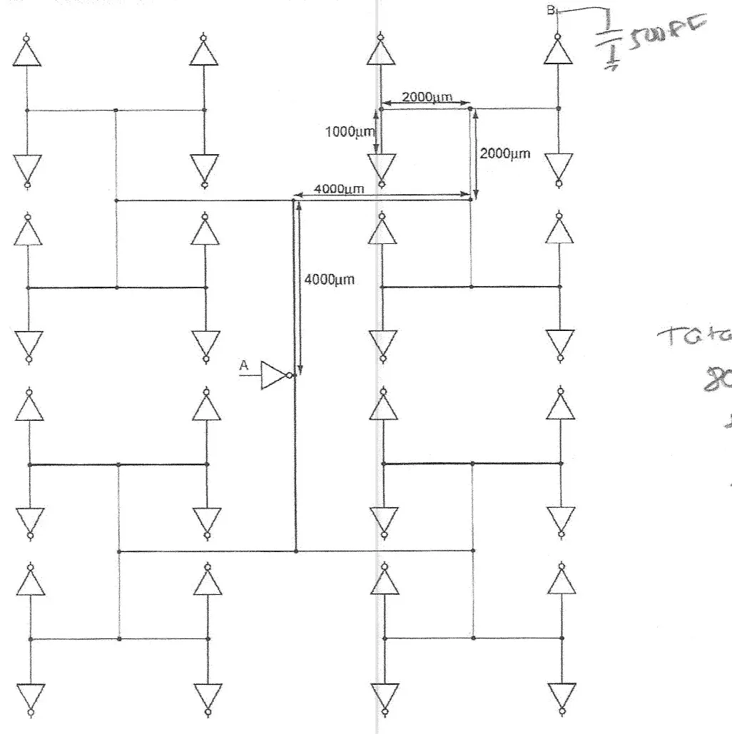— FN17-3’s H-tree (Final 2017, p5, redrawn): a root inverter at A drives 32 leaf inverters through five levels of wire; the 500 fF at B, the top-right leaf’s output, is the key’s handwriting.

The exam’s own figure (FN17-3, p5)

The printed H-tree with 32 leaf inverters, the root inverter at A, dimension arrows 4000um, 4000um, 2000um, 2000um and 1000um; handwritten: a 500fF capacitor at B and a partly visible note 'Total…' at the right. — FN17-3, p5 (source figure). The 500 fF capacitor at B and the “Total wire length” note are the key’s handwriting.

Let the fanout-of-one delay be given by $\tau_{inv} = 100$ psec. Let the gate capacitance per unit width be 2 fF/µm. Let all of the wires have a capacitance per unit length of $\mathcal{C} = 0.2$ fF/µm and a resistance per unit length of $\mathcal{R} = 0.1\ \Omega/\mu$ m. Let the inverter have a pFET width of 200 µm and an nFET width of 100 µm.

Reading the figure and the data. The root inverter’s output joins the middle of the vertical trunk, which runs 4000 µm up and 4000 µm down. At each trunk end a horizontal wire runs 4000 µm each way; at each of those four ends a vertical wire 2000 µm each way; at each of those eight ends a horizontal wire 2000 µm each way; at each of those sixteen ends a vertical stub 1000 µm each way, ending in a leaf inverter: 32 leaves. B is the output of the top leaf in the right-hand column. Every inverter, root and leaves, has the stated 200 µm + 100 µm of gate. The paper prints no load at B; the 500 fF at B is handwritten on the figure by the key’s author, and the page uses it (the key’s own arithmetic uses a different load: see the KeyNote of (a)).

Part (a): the total delay from A to B (11 points)

FN17-3a, p7. Calculate the total delay from A to B. Use Elmore delay to estimate the interconnect delay. Do not consider resistive shielding to calculate buffer delay. Ignore wire inductance. (11 points)

FN17-3's H-tree: a root inverter at A, a 4000 µm trunk each way, then 4000, 2000, 2000 and 1000 µm branches to 32 leaf inverters; B with 500 fF at the top right. — FN17-3’s H-tree (p5, redrawn): 32 leaves; B at the top right. Original figure ↑

Hint

The signal passes three things in series on its way from A to B. What does each of them have to charge?

What it asks. One number, the time from A switching to B switching, made of three pieces: the root inverter charging the tree, the wire’s own Elmore delay along the path to B’s leaf inverter, and that leaf inverter driving B. “Use Elmore delay … for the interconnect” sets the method for the middle piece; “do not consider resistive shielding to calculate buffer delay” sets the root’s load to the whole tree.

The idea. The root inverter sees one big capacitor, all 104,000 µm of wire and all 32 leaf inputs: a gate delay with a 40 pF load. On the wire, each path segment’s resistance carries half its own capacitance and everything beyond it, which in an H-tree includes a whole side subtree at every node. The three pieces are in series, so they add.

Why this formula. $T_{A\to B} = \tau_{inv}\dfrac{C_{tree}}{C_{in}} + \sum_k R_k\big(\tfrac12C_k + C_{down,k}\big) + \tau_{inv}\dfrac{C_B}{C_{in}}$ .

Where it comes from. Each gate delay is Chapter 7’s $\tau_{inv}\,C_{load}/C_{in}$ ; the wire term is Chapter 20’s segment form, measured from the root buffer’s output (its own resistance is already in the first term).
Conditions. Grounded capacitance, uniform segments, one pole; no resistive shielding for the buffers (as told); no inductance (as told). Every inverter is the same size, so $C_{in}$ is the same for the root and the leaves.
Why the whole tree loads the root. The root inverter charges every node of the tree, including the half that does not lead to B, so all of it is its load. But that half shares no wire resistance with B’s path: it appears in the first term and not in the second.
The tempting alternatives. Counting one branch per level per quarter (64,000 µm). Giving each path segment only $\tfrac12R_kC_k$ of its own and forgetting that the path’s later wire charges through it too. Putting the side subtrees’ own resistance into the sum.

A horizontal line from a root inverter with input A through five wire segments to a leaf inverter whose output is B, with 500 fF to ground. Under the segments: 4000 µm, 400 ohm, 800 fF; 4000 µm, 400 ohm, 800 fF; 2000 µm, 200 ohm, 400 fF; 2000 µm, 200 ohm, 400 fF; 1000 µm, 100 ohm, 200 fF. Over them, C_down,k: 19200, 8800, 4000, 1600, 600 fF. Dashed stubs hang boxes from the nodes: 52000 µm + 16 gates at the root; then 24000 µm + 8 gates (9600 fF), 10000 µm + 4 gates (4400 fF), 4000 µm + 2 gates (2000 fF), 1000 µm + 1 gate (800 fF). The leaf input is 600 fF. Below: script R = 0.1 ohm/µm, script C = 0.2 fF/µm, gate = 300 µm × 2 fF/µm = 600 fF. — FN17-3a’s path from A to B, unrolled added (segment lengths not to scale). Each path segment carries half its own capacitance and all of $C_{down,k}$ , the capacitance beyond it (values over the segments). The dashed boxes are the subtrees that leave the path at each node, lumped there: their wire plus their leaf gates. The lower half of the tree (52 000 µm and 16 gates, 20 000 fF) hangs at the root node and shares no resistance with B’s path.

FN17-3a

Count the wire. Because every level doubles the number of branches: the trunk, $2 \times 4000 = 8000$ µm; level 2, $4 \times 4000 = 16{,}000$ ; level 3, $8 \times 2000 = 16{,}000$ ; level 4, $16 \times 2000 = 32{,}000$ ; the leaf stubs, $32 \times 1000 = 32{,}000$ . In all 104,000 µm, ending in 32 leaf inverters.
One gate. Because the gate capacitance is per width, each inverter’s input is $(200 + 100) \times 2 = 600$ fF.
The root buffer. Because it charges the whole tree with no shielding, its load is $32 \times 600 + 0.2 \times 104{,}000 = 19{,}200 + 20{,}800 = 40{,}000$ fF, 40 pF, and its delay is $100\ \text{ps} \times 40{,}000/600 = 6666.7$ ps $= 6.667$ ns.
B’s path. Because the path runs up the trunk, right, up, right and up the stub, its segments are 4000, 4000, 2000, 2000 and 1000 µm: $R_k = 400, 400, 200, 200, 100\ \Omega$ and $C_k = 800, 800, 400, 400, 200$ fF.
What lies beyond each segment. Because at each node one subtree leaves the path: beyond the stub is B’s leaf input, 600 fF; beyond the level-4 wire, the stub (200), the leaf (600) and the other stub with its leaf (800): 1600 fF; beyond the level-3 wire, 400 + 1600 + the other level-4 half (4000 µm and 2 gates, 2000 fF): 4000 fF; beyond the level-2 wire, 400 + 4000 + the other level-3 branch (10,000 µm and 4 gates, 4400 fF): 8800 fF; beyond the trunk’s upper half, 800 + 8800 + the other level-2 quarter (24,000 µm and 8 gates, 9600 fF): 19,200 fF.
The wire’s Elmore delay. $400 \times (400 + 19{,}200) = 7.84$ ns; $400 \times (400 + 8800) = 3.68$ ns; $200 \times (200 + 4000) = 0.84$ ns; $200 \times (200 + 1600) = 0.36$ ns; $100 \times (100 + 600) = 0.07$ ns. The sum is 12.79 ns.
The leaf buffer. Because B’s leaf drives the 500 fF at B, $100 \times 500/600 = 83.3$ ps.
Add. $6.667 + 12.79 + 0.083 = 19.54$ ns.

Check. Regroup the wire’s sum the key’s way, by capacitance, to see each piece by a different route. The path segments against their own wire, $\tfrac12\mathcal{R}\mathcal{C}L^2$ each: $0.16 + 0.16 + 0.04 + 0.04 + 0.01 = 0.41$ ns. The four side subtrees through the path resistance up to their nodes: $400 \times 9600$ , $800 \times 4400$ , $1000 \times 2000$ , $1200 \times 800$ Ω·fF $= 3.84 + 3.52 + 2 + 0.96 = 10.32$ ns. B’s leaf input through all 1300 Ω: 0.78 ns. And the path’s own wire through the path resistance before each segment: $800 \times 400 + 400 \times 800 + 400 \times 1000 + 200 \times 1200$ Ω·fF $= 1.28$ ns. The total is $0.41 + 10.32 + 0.78 + 1.28 = 12.79$ ns, the same. A bound agrees: the 19.2 pF beyond the trunk lies behind 400 to 1300 Ω, and the trunk’s own 0.8 pF behind less than 400 Ω, so the wire delay lies between $19.2\ \text{pF} \times 400\ \Omega = 7.68$ ns and $20\ \text{pF} \times 1300\ \Omega = 26$ ns.

Answer: $T_{A\to B} = 6.667 + 12.79 + 0.083 = 19.54$ ns: the root buffer 6.667 ns, the wire 12.79 ns (65.5 %), the leaf buffer 83.3 ps.

Remember. A clock tree’s delay is buffer + wire + buffer. The root buffer charges everything; the wire sum counts, at each node, the subtree that leaves there. In an H-tree most of the wire delay is the first segment, which carries half the tree.

The answer key differs

It gives 17.48 ns (

5.33 + 11.82 + 0.333

), with six slips, each re-derived from its own inputs. (1) Wire count. Its

8000 + 8000 + 8000 + 4(4000 + 4000 + 2000) = 64{,}000

µm counts one branch per level in each quarter; the figure has 104,000 µm. (2) Root buffer denominator. It writes 200 µm, but its 5.33 ns needs 300 µm (600 fF); with 200 µm and its own 64,000 µm it would be 8 ns. With the figure’s wire it is 6.667 ns. (3) The path’s own wire. Its

\tfrac12\mathcal{R}\mathcal{C}L^2

terms count each path segment only against itself, so the later path wire charging through the earlier segments, 1.28 ns, is missing. (4) Two decimal slips in those terms:

\tfrac12\mathcal{R}\mathcal{C}(2000\ \mu\text{m})^2 \times 2

is 0.08 ns, not 0.8, and

\tfrac12\mathcal{R}\mathcal{C}(1000\ \mu\text{m})^2

is 0.01 ns, not 0.1. (5) The last term,

\mathcal{R}(13{,}000\ \mu\text{m})(600\ \text{fF})

, is 0.78 ns, not 0.28. Its side-subtree terms, 3.84, 3.52, 2 and 0.96 ns, are right. With (4) and (5) fixed its grouping gives 11.51 ns, and with (3) added, 12.79 ns. (6) The leaf load. It writes

(1000\ \mu\text{m}/300\ \mu\text{m})\tau_{inv}

, a load of 1000 µm of gate (2000 fF, 333 ps), where its own figure has 500 fF (83.3 ps). The total is 2.06 ns more than its 17.48.

Part (b): jitter from supply noise (11 points)

FN17-3b, p7. If the buffers have a power-supply sensitivity of $(V_{DD}/\tau_{inv})(\partial\tau_{inv}/\partial V_{DD}) = -0.1$ and operate at a nominal supply voltage of 1.2 V, what jitter can one expect from power supply noise that is 10% of the nominal supply voltage. (11 points)

FN17-3a's path unrolled: the root inverter, five wire segments with their side subtrees, the leaf inverter and B's 500 fF. — FN17-3a’s path (added): two buffers (the silicon) and five wire segments between them. Original figure ↑

The same question on FN10-6c (fs1, redrawn): a clock tree’s latency moves with its supply, and the moving edge is the jitter. Original figure ↗

Hint

Which parts of the 19.54 ns change when the supply moves?

What it asks. How far the clock edge at B moves in time when the supply moves by 10 % of 1.2 V, that is, by 0.12 V, from cycle to cycle. That movement is the jitter. The given sensitivity $S = -0.1$ is a ratio of fractional changes. What must be decided first is which delays it applies to: the words “the buffers have a power-supply sensitivity” name them.

The idea. A buffer’s delay is charge over current, and its current depends on its supply, so a lower supply makes it slower. The wire’s Elmore delay depends only on its resistance and capacitance, set by metal and dielectric, so it does not move. So only the two buffers on B’s path, the root (6.667 ns) and the leaf (83.3 ps), change, each by the same fraction $S \times \Delta V_{DD}/V_{DD} = (-0.1)(-0.1) = 1$ %. If the supply moves by that much from one cycle to the next, the edge at B moves by 1 % of 6.75 ns.

Why this formula. $\Delta\tau \approx S\,\tau_{silicon}\,\Delta V_{DD}/V_{DD}$ .

Where it comes from. The definition of $S$ , with the derivative replaced by a difference: $\Delta\tau/\tau \approx S\,\Delta V_{DD}/V_{DD}$ (Chapter 21 §8). It is the first term of a Taylor expansion, good for small changes; 10 % is at the edge of “small”, and the paper asks for the estimate.
Conditions. The sensitivity is the same for every buffer (they are identical) and the noise reaches every buffer on the path. The wire’s RC is independent of the supply.
How “10 % noise” is read. Noise “that is 10 % of the nominal supply” names its size, 0.12 V. Read as a supply that moves over 0.12 V (a 10 % droop and back), the edge moves over $1\ \% \times 6.75$ ns. This is the reading FN10-6c’s key and fs1 use (a supply “varying between 2.5 and 2.0 V” gives the edge’s range), and the reading the key uses here; FN17-1b on the same paper uses “10 % droop” for a one-sided fall, which supports it. Read as ±10 % (0.12 V either way, a 0.24 V swing), the edge’s range doubles.
The tempting alternative. Applying $S$ to the whole 19.54 ns: that gives 195.4 ps, nearly three times too much, because two-thirds of the path is wire.

FN17-3b

The silicon delay. Because only the buffers depend on the supply, take (a)‘s root buffer and leaf buffer: $6666.7 + 83.3 = 6750$ ps. The 12.79 ns of wire is left out.
The fractional change. Because the noise is 10 % of 1.2 V, $\Delta V_{DD}/V_{DD} = 0.12/1.2 = 0.1$ .
The delay change. Because $\Delta\tau \approx S\,\tau_{silicon}\,\Delta V_{DD}/V_{DD}$ , a 10 % droop gives $(-0.1) \times 6750 \times (-0.1) = +67.5$ ps: the root buffer 66.67 ps and the leaf 0.83 ps.
As jitter. Because the noise comes and goes from cycle to cycle, the edge at B arrives up to 67.5 ps late on a drooped cycle and on time on a clean one: it wanders over 67.5 ps.

Check. Without the linearization added: if $S$ stays constant over the swing, the delay goes as $V_{DD}^{S}$ , so a 10 % droop multiplies the 6.75 ns by $0.9^{-0.1} = 1.0106$ , +71.5 ps, and a 10 % rise by $1.1^{-0.1}$ , −64.0 ps (a 135.5 ps range). The first-order 67.5 ps is about 6 % low, as fs1’s FN10-6c curve also shows (133 against 100 ps). FN10-6c is the same rule on other numbers (fs1): $0.25 \times 0.2 \times 2$ ns $= 100$ ps there; its $|S| \times \Delta V/V$ , 0.05, is five times this tree’s 0.01, which outweighs this tree’s 3.4 times larger latency.

Answer: about 67.5 ps of jitter at B: 1 % ( $S \times \Delta V/V = 0.1 \times 0.1$ ) of the 6.75 ns of buffer delay; the wire’s 12.79 ns does not change. This is the answer for noise read as a 10 % (0.12 V) change of the supply. If the noise is ±10 % about nominal, the edge moves ±67.5 ps, a 135 ps range.

Remember. Jitter ≈ |S| × (fractional supply change) × (silicon latency): buffers only, wires never. Say how you read “x % noise”.

The answer key differs

It writes the same method,

0.1 \times 0.1 \times 5.66

= 56.6

ps, with the buffers only (5.33 + 0.333 ns), and reads the noise one-sidedly, as here. Its 5.66 ns carries (a)‘s slips: the 64,000 µm of wire in the root buffer’s load and the 2000 fF leaf load. With the figure’s 104,000 µm and 500 fF the buffer delay is 6.75 ns and the jitter 67.5 ps.

Part (c): should inductance be included? (points illegible)

FN17-3c, p7 (the second page labelled 7). If the inductance per unit length for these wires is $L = 0.1$ nH/mm, should inductance be included in the interconnect delay analysis? Please explain. [The point value is overwritten and illegible.]

When inductance matters (Chapter 21, Lecture20 @ 49:37, redrawn): only between

\ell_1

and

\ell^{*}

, where the time of flight is above both the RC delay and the slew. Original figure ↗

Hint

Where do the RC and LC delays of these wires cross, and how long is the shortest wire in the tree?

What it asks. A yes or no with a reason: does the wire’s inductance change the delay of this clock tree enough that the analysis must include it? The paper writes the inductance per length as $L$ ; this page writes it $\mathcal{L}$ , because $L$ is a length in part (a). The unknown is a comparison of three times, and the paper gives no edge (slew) time, which is the decision to make.

The idea. A wire with inductance has two delays: the RC (diffusion) delay $\tfrac12\mathcal{R}\mathcal{C}\ell^2$ and the LC time of flight $\sqrt{\mathcal{L}\mathcal{C}}\,\ell$ . The larger governs. Inductance matters only on lengths where the time of flight is the larger and it is longer than the edges’ transition time; that window exists only if the edges are faster than $2\mathcal{L}/\mathcal{R}$ , the delay at the crossover. These wires are resistive: 0.1 Ω/µm is 100 Ω per mm. Expect the crossover at a short length and a tiny delay.

Why this formula. $\ell^{*} = 2\sqrt{\mathcal{L}\mathcal{C}}/(\mathcal{R}\mathcal{C})$ and $t_{RC}(\ell^{*}) = t_{LC}(\ell^{*}) = 2\mathcal{L}/\mathcal{R}$ , against the edge time.

Where it comes from. Equate the board’s two delays (Chapter 21 §7): $\tfrac12\mathcal{R}\mathcal{C}\ell^2 = \sqrt{\mathcal{L}\mathcal{C}}\,\ell$ gives $\ell^{*}$ ; putting it back gives $2\mathcal{L}/\mathcal{R}$ .
Conditions. Uniform wires with a controlled return; an order-of-magnitude comparison. Units: with $\mathcal{R}$ in Ω/mm and $\mathcal{C}$ in pF/mm, $\mathcal{R}\mathcal{C}$ is in ps/mm².
No slew time given. Chapter 21 §7, step 5, gives two ways round it: (a) a wire much longer than $\ell^{*}$ is an RC line whatever the slew, because the larger delay governs; (b) an edge takes at least about one FO1 delay, so if $\tau_{inv} \gg 2\mathcal{L}/\mathcal{R}$ inductance cannot matter.
The tempting alternative. Comparing $\omega L$ with $R$ for the whole tree at an arbitrary frequency, or assuming a slew time without saying why.

A log-log plot of time against wire length. A steep line t_RC and a shallower line t_LC cross at 0.447 mm and 2 ps, marked 2L/R = 2 ps. A dashed horizontal t_slew at 200 ps meets t_LC at 44.7 mm, marked l_1 with a dotted guide. A dotted vertical at 13 mm marks t_RC = 1690 ps and t_LC = 58.1 ps. — FN17-3’s wires added (computed from $\mathcal{R} = 100\ \Omega$ /mm, $\mathcal{C} = 0.2$ pF/mm, $\mathcal{L} = 0.1$ nH/mm): the RC diffusion time grows as $\ell^2$ , the LC flight time as $\ell$ , and they cross at $\ell^{*} = 0.447$ mm, 2 ps. A window opens only where the flight time beats both the RC delay ( $\ell < \ell^{*}$ ) and the slew ( $\ell > \ell_1 = t_{slew}/\sqrt{\mathcal{L}\mathcal{C}}$ ). With the key’s 200 ps slew (dashed), $\ell_1 = 44.7$ mm, far beyond $\ell^{*}$ , so there is no window; it would take an edge faster than 2 ps. At the path’s 13 mm, $t_{RC} = 1690$ ps against $t_{LC} = 58.1$ ps.

FN17-3c

Per-millimetre values. Because the inductance is per mm, convert the rest: $\mathcal{R} = 0.1\ \Omega/\mu\text{m} = 100\ \Omega$ /mm and $\mathcal{C} = 0.2$ fF/µm $= 0.2$ pF/mm.
The time of flight. $\sqrt{\mathcal{L}\mathcal{C}} = \sqrt{0.1 \times 10^{-9} \times 0.2 \times 10^{-12}}$ s/mm $= 4.472$ ps/mm.
The crossover. $\ell^{*} = 2 \times 4.472/(100 \times 0.2) = 0.447$ mm, where both delays are $2\mathcal{L}/\mathcal{R} = 2 \times 0.1\ \text{nH}/100\ \Omega = 2$ ps.
Route (a), the lengths. Because the shortest wire in the tree, a leaf stub, is 1 mm, more than twice $\ell^{*}$ , every wire is an RC line: the stub’s RC delay is 10 ps against a 4.47 ps flight; a 4 mm wire’s, 160 ps against 17.9 ps; the 13 mm path’s, 1690 ps against 58.1 ps.
Route (b), the edges. Because an edge takes at least about one FO1 delay, 100 ps, the edges are 50 times slower than 2 ps: no window opens at any length.
Decide. No: inductance can be left out.

Check. The same test in frequency, the key’s route: a wire’s $j\omega\mathcal{L}$ reaches its $\mathcal{R}$ only at $\omega = \mathcal{R}/\mathcal{L} = 100\ \Omega/0.1\ \text{nH} = 10^{12}$ rad/s, about 159 GHz. An edge of 100–200 ps has its frequency content below about $1/t_{slew}$ , a few to ten gigahertz, more than ten times lower, where the wire is all resistance. And $\ell^{*}$ is the distance the wave travels in $2\mathcal{L}/\mathcal{R}$ : $(2\ \text{ps})/(4.472\ \text{ps/mm}) = 0.447$ mm, as step 3 found.

Answer: no. With these wires the RC and LC delays cross at $\ell^{*} = 0.447$ mm, where both are only $2\mathcal{L}/\mathcal{R} = 2$ ps. Every wire in the tree (1 to 4 mm) is much longer, so its RC delay dominates the time of flight, and the edges (at least $\tau_{inv} = 100$ ps) are far slower than 2 ps, so no transmission-line window exists.

Remember. Compute $\ell^{*}$ and $2\mathcal{L}/\mathcal{R}$ first. Resistive wires (tens of Ω per mm or more) have a tiny window; inductance is a matter for wide, thick, low-resistance top-level wires with fast edges.

The answer key agrees

It compares

\omega = \mathcal{R}/\mathcal{L} = (0.1)(1000)/(0.1 \times 10^{-9}) = 10^{12}

rad/s, 159 GHz, with the content of a slew it takes as about 200 ps, and concludes that inductance does not matter: the frequency form of route (b). Its 200 ps is assumed, not given; route (a) needs no slew at all.

Harder variations: clock-tree wires

You need

FN17-3’s tree (part (a)). 104,000 µm of wire at 0.1 Ω/µm and 0.2 fF/µm, 32 leaf inverters of 600 fF each (300 µm of gate at 2 fF/µm), $\tau_{inv} = 100$ ps. The root buffer drives 40 pF in 6.667 ns; the wire to any leaf’s input is 12.79 ns by the segment form (path segments 400, 400, 200, 200, 100 Ω with $C_{down}$ = 19,200, 8800, 4000, 1600, 600 fF); a leaf into 500 fF takes 83.3 ps. Total to B: 19.54 ns.

FN17-3a's path unrolled: the root inverter, five wire segments with their C_down and side subtrees, the leaf inverter and B's 500 fF. — FN17-3a’s path, unrolled (added). Original figure ↑

A chain of inverters (Chapter 8 §4). $N$ inverters from $C_{in}$ to $C_{out}$ have path effort $F = C_{out}/C_{in}$ ; equal gains $f = F^{1/N}$ give the least delay, $N F^{1/N}\tau_{inv}$ , best near $N = \ln F$ ; inverters are added in pairs so that the logic is not inverted.

Jitter (Chapter 21 §8). $\Delta\tau \approx S\,\tau_{silicon}\,\Delta V/V$ , buffers only. Between two leaves, what matters is the part of their paths they do not share.

These two variations added go beyond FN17-3 in the ways the real midterm did: each is a chain of five parts across three chapters (7, 8 and 20, with 21’s jitter), Variation 4 redesigns the root, and Variation 5 asks for a skew fix in a setup no past paper uses. The budgets assume the practice finals’ pace. No key exists, so there is no key verdict.

Variation 4: a buffer chain at the root (about 20 minutes)

Variation 4: a buffer chain at the root

added The question. In FN17-3’s tree, replace the single root inverter by a chain of inverters sized by Chapter 8’s method, the first of them the original inverter (so A’s load is unchanged) and the last driving the tree. Keep resistive shielding out, as the paper does. The chain must not invert the clock at the leaves. (a) What path effort does the chain face? (b) How many stages, with what gain, and what is the chain’s delay? (c) Size every stage. (d) What is the new delay from A to B, and what share of it is wire? (e) What jitter does FN17-3b’s 10 % supply noise now give?

FN17-3's H-tree: a root inverter at A, 32 leaf inverters, B at the top right with 500 fF. — FN17-3’s tree (p5, redrawn): only the root inverter changes. Original figure ↑

A chain from input A through five inverters in a row, labelled C1 to C5 above and 600, 1390, 3219, 7456 and 17 269 fF below, with f = 2.316 above the chain. The last inverter drives a box labelled C_tree, 40 pF = 32 × 600 fF + 0.2 × 104 000 fF. Below: F = 66.67, N = 5, 5 f tau_inv = 1158.1 ps. — Variation 4 added: FN17-3’s root inverter replaced by five inverters sized by Chapter 8’s method. Each stage’s input is 2.316 times the one before ( $f = 2.316$ is the gain per stage), from the original 600 fF to 17 269 fF, and the last drives the tree’s 40 pF (32 leaf inputs of 600 fF plus 104 000 µm of wire at 0.2 fF/µm). The path effort is 66.67; five stages (an odd number keeps the clock’s polarity) give 1158.1 ps against the single inverter’s 6666.7 ps. The inverters are drawn equal; their sizes are in the labels.

Hint

The chain replaces one inverter. How many inverters can it have without turning the clock upside down?

What it asks. A redesign of the biggest silicon delay in FN17-3a, the root buffer’s 6.667 ns, with Chapter 8’s sizing; then its effect on the total and on the jitter. What is new is joining Chapter 8’s chain to Chapter 20’s tree: the chain’s load is the tree, and the wire’s delay after it does not change.

The idea. One 600 fF inverter driving 40 pF has a gain of 66.7: far too much for one stage. A chain of growing inverters spreads that gain over several stages, each near 2.7–4, and the delay falls to a few FO1 delays per stage. The chain must keep the clock’s polarity, so it has an odd number of stages (1, 3, 5, …). The wire’s Elmore delay is measured from the last stage’s output and is unchanged; so the wire, 12.79 ns, becomes almost the whole delay, and the jitter, which only sees silicon, falls with the chain’s delay.

Why this formula. Chapter 8’s $\text{Delay} = N F^{1/N}\tau_{inv}$ with $F = C_{tree}/C_{in}$ .

Where it comes from. Each stage’s delay is its gain times $\tau_{inv}$ (Chapter 7); with fixed $F$ the sum of gains is least when they are equal (Chapter 8 §3), and the best $N$ is near $\ln F$ (§4).
Conditions. Inverters only ( $g = 1$ ), no branching inside the chain, no parasitic delay (the course’s model), the load lumped (no shielding, as the paper says). The first stage’s size is fixed by A’s load.
The tempting alternatives. An even number of stages (4 is 15 ps faster here but delivers an inverted clock). Sizing with $f = 4$ by habit instead of comparing the odd counts. Counting the wire’s 20.8 pF out of the chain’s load.

Variation 4

(a) The path effort. Because the chain’s first input is the original 600 fF and its load is the whole tree, $F = 40{,}000/600 = 66.67$ , and $\ln F = 4.20$ .
(b) The stage count. Because only odd counts keep the clock’s sense, compare $N F^{1/N}\tau_{inv}$ for 1, 3, 5 and 7: 6666.7, 1216.4, 1158.1 and 1275.4 ps. Five stages, with a gain of $66.67^{1/5} = 2.316$ each, 231.6 ps a stage: 1158.1 ps.
(c) The sizes. Because every stage has the same gain, each input is 2.316 times the one before: 600, 1390, 3219, 7456 and 17,269 fF, and the last drives 40,000 fF. At 2 fF/µm the last inverter has 8635 µm of gate (a third nFET, two-thirds pFET, as the original).
(d) The new total. Because the wire and the leaf are unchanged, $T_{A\to B} = 1.158 + 12.79 + 0.083 = 14.03$ ns, 5.51 ns faster than 19.54 ns. The wire is now 91.2 % of the delay.
(e) The jitter. Because only silicon moves, $\Delta\tau = 0.1 \times 0.1 \times (1158.1 + 83.3)$ ps $= 12.4$ ps (24.8 ps for ±10 %), 5.4 times less than FN17-3b’s 67.5 ps.

Check. A bound: over any real number of stages, $N F^{1/N}\tau_{inv}$ is least at $N = \ln F = 4.2$ , where it is $e\,\ln F\,\tau_{inv} = 1141.6$ ps. No chain beats it, and five stages are 1.4 % above it.

Answer: (a) $F = 66.67$ . (b) Five stages, gain 2.316, 1158.1 ps. (c) Inputs 600, 1390, 3219, 7456, 17,269 fF. (d) 14.03 ns, of which 91.2 % is wire. (e) 12.4 ps (from 67.5 ps).

Remember. A single inverter driving a clock tree is the slowest and the noisiest choice. Size the root as a chain with an odd number of stages; then the wire dominates, and widening the trunk (whose segment carries half the tree) is the next lever.

Variation 5: two leaves, two loads, and two ways to fix the skew (about 25 minutes)

Variation 5: two leaves, two loads, and two ways to fix the skew

added The question. In FN17-3’s tree, let B′ be the other leaf on B’s last branch: the inverter on the 1000 µm stub that points down from the node where B’s stub points up. B keeps its 500 fF; B′ drives 2 pF. (a) What is the wire’s Elmore delay to B′‘s leaf input? (b) Find the arrival times at B and B′ and the skew between them. (c) With FN17-3b’s sensitivity ( $S = -0.1$ ), how far does a 10 % droop of the whole tree’s supply move each edge, and the skew? (d) What if the droop hits only the root buffer, or only B′‘s leaf inverter? (e) Two fixes for the skew: (i) make B′‘s leaf inverter four times larger; (ii) add 1.5 pF of load at B. Find the arrival times and the skew with each, and say which is better.

FN17-3's H-tree: 32 leaf inverters in four columns; B at the top of the right column. — FN17-3’s tree (p5, redrawn): B′ is the inverter just below B’s, on the other stub of the same node. Original figure ↑

Three pairs of rising-step waveforms, B above B′, on one time axis in ns broken between 20.0 and 21.9. Top pair: B rises at 19.540 and B′ at 19.790, a 250 ps dimension between them. Pair (i): B rises at 22.000 and B′ at 22.180, 180 ps apart. Pair (ii): B and B′ both rise at 19.790, joined by a dotted line labelled 0. — Variation 5 added, computed from FN17-3’s three pieces for each leaf (root buffer, wire, leaf buffer). Top pair: B (500 fF) and B′ (2 pF) arrive 250 ps apart, all of it from the leaf loads. (i) Making B′‘s leaf inverter four times larger puts 1800 fF more on the tree: both leaves arrive about 2.46 ns later and the skew is still 180 ps. (ii) Padding B’s load to 2 pF brings both to 19.790 ns, with no skew and nothing upstream changed. The time axis is broken between 20.0 and 21.9 ns.

Hint

B and B′ share every wire segment but the last stub. What in their two paths is different, and what does resizing a leaf do to the tree?

What it asks. A skew analysis between two clock leaves with different loads, then its behaviour under supply noise, then a design choice. What is unfamiliar is that a fix at a leaf can feed back into the tree.

The idea. An H-tree is built so that every leaf is the same wire distance from the root: by symmetry, the wire’s Elmore delay to every leaf input is the same 12.79 ns. So the skew between B and B′ comes only from what differs: their leaf buffers’ loads. Supply noise that is common to the tree moves both edges almost equally; only the silicon they do not share moves the skew. A fix at B′‘s input changes the tree’s capacitance, which every wire segment upstream must charge; a fix at B’s output (its load) changes nothing upstream.

Why this formula. The three pieces of FN17-3a for each leaf, $t_{root} + T_{wire} + \tau_{inv}C_{leaf}/C_{in,leaf}$ , and the jitter rule $\Delta\tau \approx S\,\tau\,\Delta V/V$ on each buffer.

Where it comes from. Chapter 7’s gate delay for the buffers, Chapter 20’s segment form for the wire, Chapter 21’s first-order supply rule (FN17-3b).
Conditions. As FN17-3a. A larger leaf inverter has a proportionally larger input (2400 fF for four times the size) and drives in proportion ( $\tau_{inv}C_{load}/C_{in}$ with the new $C_{in}$ ).
The tempting alternatives. Upsizing B′‘s inverter and recomputing only its own delay, forgetting that its larger input sits on the tree. Treating common supply noise as skew.

Variation 5

(a) The wire to B′. Because B′‘s path shares the first four segments with B’s and its own stub is the same 1000 µm into the same 600 fF, and the other stub (now B’s) is the side branch at that node, the sum is the same: $7.84 + 3.68 + 0.84 + 0.36 + 0.07 = 12.79$ ns. By the H-tree’s symmetry it is the same to every leaf.
(b) Arrivals and skew. Because B′‘s leaf inverter drives 2 pF, it takes $100 \times 2000/600 = 333.3$ ps against B’s 83.3 ps: B arrives at 19.540 ns, B′ at 19.790 ns. The skew is 250 ps, all of it from the leaf loads.
(c) Common noise. Because every buffer slows by 1 % in a 10 % droop, B moves by $0.01 \times (6666.7 + 83.3) = 67.5$ ps and B′ by $0.01 \times (6666.7 + 333.3) = 70$ ps: each edge jitters by about 70 ps, but the skew changes by only 2.5 ps, 1 % of the 250 ps difference.
(d) Local noise. Because the root buffer is shared, a droop there alone moves both edges by 66.7 ps and the skew by nothing. A droop at B′‘s leaf alone moves only B′, by $0.01 \times 333.3 = 3.3$ ps. Between two leaves, the jitter that matters comes from the silicon they do not share.
(e i) Upsize B′‘s leaf. Because its input becomes 2400 fF, the tree gains 1800 fF at B′‘s input. The root’s load becomes 41.8 pF: 6966.7 ps (+300 ps). Every path segment to B and B′ carries the extra 1800 fF: B’s wire becomes 14.95 ns (+1800 fF × the 1200 Ω it shares with B′‘s path, 2.16 ns), B′‘s 15.13 ns (+2.34 ns). B′‘s leaf now drives 2 pF from 2400 fF in 83.3 ps. Arrivals: B at 22.000 ns, B′ at 22.180 ns: the skew is still 180 ps. And B’s arrival moved 2.46 ns, while a leaf in the lower half, which shares none of B′‘s path, moves only 0.30 ns (the root’s share): (i) skews B’s corner by about 2.2 ns against the rest of the tree.
(e ii) Pad B’s load. Because B’s leaf output is not part of the tree, adding 1.5 pF there changes only B’s leaf delay, to 333.3 ps: both arrive at 19.790 ns, skew 0, and no other leaf moves.

Check. In (e i), the skew that remains is exactly the difference of the two last stubs: B′‘s stub now carries $100 \times (100 + 2400)$ Ω·fF $= 250$ ps against B’s 70 ps, a 180 ps difference, while the leaf delays are equal. That is the price of putting a large input at the end of a resistive stub. In (e ii), both leaves have the same wire and the same leaf load, so the skew must be zero.

Answer: (a) 12.79 ns, the same as to B. (b) B 19.540 ns, B′ 19.790 ns: skew 250 ps. (c) 67.5 and 70 ps; the skew moves 2.5 ps. (d) Root only: both 66.7 ps, skew unchanged; B′‘s leaf only: 3.3 ps. (e) (i) 22.000 and 22.180 ns, skew 180 ps, but B’s corner now about 2.2 ns late against the lower half of the tree; (ii) both 19.790 ns, skew 0: pad the light leaf’s load.

Remember. In a balanced tree, skew comes from what the leaves do not share. Fix it where it does not feed back: balance the leaf loads (or the stub wires), not the leaf inverters’ inputs, which the whole tree must charge.

How to approach a power-grid or decap question

Recognize it by the words, not a picture: these are short-answer questions with no figure. The prompts are “why are grids preferred for power-ground distributions”, “name at least three sources of on-chip decoupling capacitance”, “why is on-chip decoupling capacitance necessary for power-supply integrity”, “what is a reasonable decoupling capacitance target to ensure no more than a 10% droop”. Each is worth 5 to 7 points. FN12 gives 180 minutes for 200 points, about 0.9 minutes a point, so each answer gets about 4.5 to 6.3 minutes: a few ranked lines and one number.

The model (Chapter 21 §8–§12). Every gate assumes that its supply, the difference between $V_{DD}$ and ground, holds still. Two things move it.

DC, IR drop. The chip draws an average current $I$ through the resistance $R$ of the wiring from the pads to the gate, so the gate sees $V_{DD} - IR$ . The cause is resistance.
AC, $L\,dI/dt$ noise. The current changes fast at every clock edge, and the wiring and the package have inductance $L$ ; a changing current through an inductance induces $L\,dI/dt$ . The cause is inductance.

Two defences answer the two causes. A grid of $V_{DD}$ and ground straps gives many parallel paths, so both the resistance and the inductance to every point are small (§9). Decoupling capacitance (decap) between $V_{DD}$ and ground, next to the circuits, supplies the fast part of the current locally, so little of it passes through the package’s inductance (§10–§12).

Interleaved V_DD and gnd straps on two layers with vias, pads at every strap end, and four thick arrows converging on a centre point X; a signal line between a V_DD and a gnd strap. — A power and ground grid (Chapter 21 §8, after the board, Lecture20 @ 55:29): many parallel paths from the pads to any point X. Original figure ↗

The supply’s path onto the chip (Chapter 21 §10, Lecture20 @ 57:57, redrawn): the package’s inductance in each rail, and the decap beside the circuits. Original figure ↗

Why these, and their conditions. Parallel paths are circuit theory: $N$ equal resistances in parallel have $1/N$ of one, and so, if they do not couple, do $N$ inductances; memorize it, and the reason a grid exists follows. $V = L\,dI/dt$ is the inductor’s law; memorize it, and estimate $dI/dt$ as the edge’s charge over its time. The charge balance is two lines; derive it: before the edge the decap holds $C_{decap}V_{DD}$ and the load nothing; after it both sit at $V_{DD} - \Delta V$ with the same total charge, $C_{decap}V_{DD} = (C_{decap} + C_{sw})(V_{DD} - \Delta V)$ . It assumes that the package delivers nothing during the edge (its inductance is too slow) and that the decap is close and fast: a decap behind a series resistance $R_s$ responds only on times longer than about $R_sC_{decap}$ (Chapter 21 §11).

The moves.

Name the noise the question is about, DC (IR drop, caused by resistance) or AC ( $L\,dI/dt$ , caused by inductance), and say which defence answers it.
“Why grids”: ranked: low $R$ and low $L$ from many redundant paths; built-in decap; signal returns. The cost: routing tracks.
“Sources of decap”: implicit metal–metal (the lowest series resistance), n-well and quiet gates; explicit thin-oxide MOS.
“Why on-chip decap”: the edge’s charge cannot come through the package’s inductance in time, so it is stored next to the circuits and refilled between edges.
“A decap target”: the charge balance, $C_{decap} \ge C_{sw}(1 - \varepsilon)/\varepsilon$ , with its assumptions stated.
One number makes each short answer convincing: one strap’s IR drop against $N$ straps’, or the edge’s $L\,dI/dt$ through the package.

Decide on the way: whether the question wants a ranked list (“most important” is what the FN12 key marks); what counts as the switching load (the whole clock net rises in each edge; the rest of the logic only on the cycles it switches); whether “10 % droop” is a fraction of $V_{DD}$ (it is).

Traps. Calling the grid’s capacitance a cost (on the supply it is decap). Listing switching gates as decap (only the quiet ones lend their input capacitance). Answering only the list in FN12-4 and not the “why”. Writing $C_{decap} = C_{sw}/\varepsilon$ , which forgets that the load keeps part of the shared charge (10 nF instead of 9). Counting a capacitor on the board as decap: it sits behind the same package inductance. Counting every nanofarad of decap as equally useful: one behind a large series resistance cannot serve a fast edge.

FN12-3: why grids for power and ground (7 points)

You need

Two kinds of supply noise (Chapter 21 §8). The supply at a gate is lower than at the pads by the IR drop, the average current times the network’s resistance (DC), and it fluctuates by $L\,dI/dt$ , the change of current times the network’s and the package’s inductance (AC). Both must be small at every point where circuits draw current, the centre of the die included, the farthest point from the pads.

Parallel paths added (circuits). $N$ equal resistances in parallel have $R/N$ ; $N$ equal inductances, if they do not couple, about $L/N$ .

A controlled return (Chapter 21 §6). A signal’s current returns along the nearest line that offers a path. If a $V_{DD}$ or ground line runs right beside the signal, the current loop is small, and so is the signal’s inductance.

Return paths of a signal: through the package at DC, through the nearest line at high frequency; and a signal wire between a gnd line and a V_DD line. — Return paths (Chapter 21 §6, redrawn): at high frequency the return current flows in the nearest line. Original figure ↗

The question (FN12-3, p3, in the paper’s words). Why are grids preferred for power-ground distributions? Provide at least two reasons. (7 points)

Why a grid added (FN12-3 has no figure). (a) One strap from an edge pad to a load at the centre of the die: all the current $I$ flows through one strap’s resistance $R$ and inductance $L$ . (b) A grid of $V_{DD}$ and ground straps on two metal layers, joined by vias where like-named straps cross and fed from pads on every edge: the current reaches the load along $N$ parallel paths, so the effective resistance and inductance fall to about $R/N$ and $L/N$ . The dashed line $s$ is a signal wire; its return current flows in the adjacent ground strap, which keeps its loop, and so its inductance, small.

Reading the question. “Grids” are meshes of $V_{DD}$ and ground straps, panel (b); the alternative is a few separate wires from the pads, panel (a). With 7 points, give three reasons, ranked.

Two reasons, and a third (7 points)

FN12-3, p3. Why are grids preferred for power-ground distributions? Provide at least two reasons. (7 points)

Hint

What does a gate at the centre of the die need from the supply wiring, and what happens to resistances and inductances that sit side by side?

What it asks. A comparison, in words: what a mesh of $V_{DD}$ and ground straps does better than a few separate supply wires. The unknown is a list of reasons, and the word that decides the method is “preferred”: each reason must name what the grid improves and why, not just describe the grid.

The idea. A supply network has one job: to hold $V_{DD}$ minus ground steady at every gate. It fails in two ways, by IR drop through its resistance and by $L\,dI/dt$ through its inductance. A grid connects every point to the pads through many paths at once, so the resistances and inductances of those paths sit in parallel: the more paths, the smaller both. Two more benefits come with the same metal for free: neighbouring $V_{DD}$ and ground lines form a capacitor across the supply, which is decap, and every signal wire has a supply line close by to carry its return current.

Why this formula. $R_{eff} = R_1/N$ and $L_{eff} \approx L_1/N$ , so $\Delta V_{IR} = I R_1/N$ .

Where it comes from. Resistances in parallel add as conductances; $N$ equal ones give $R_1/N$ . Inductances in parallel combine the same way if their magnetic coupling is ignored.
Conditions. The paths are about equal and share the current. Neighbouring straps do couple magnetically, so the inductance falls a little less than $1/N$ : the trend holds, the factor is approximate.
The numbers are illustrative added: one strap of 1.5 Ω from an edge pad to the centre, and circuits at the centre drawing 2 A, for example (Variation 7 uses the same chip).
The tempting alternative. One wide strap per supply. Widening a single strap lowers its resistance, but every gate still reaches the pads through that one path, and its inductance and its loop with the ground return stay large.

FN12-3

The job. Because a gate’s delay and its logic levels depend on the supply difference, the network must keep both the DC drop ( $IR$ ) and the AC noise ( $L\,dI/dt$ ) small at every point, the die’s centre included.
One strap. Because all the current flows through one path: $2\ \text{A} \times 1.5\ \Omega = 3$ V of IR drop, more than the whole 1.2 V supply. One path cannot do it.
Reason 1 (most important): low resistance and low inductance. Because a grid fed from pads on every edge reaches the centre along many parallel paths, 100 of them give $1.5/100 = 15$ mΩ and a drop of 30 mV, 2.5 % of 1.2 V. The same paths put the inductances in parallel: 1 nH per path becomes about 10 pH. The paths are also redundant: a weak via or a narrow strap does not cut any gate off.
Reason 2: built-in decap. Because a grid runs $V_{DD}$ and ground lines side by side on every layer, the capacitance between them sits right across the supply. On a signal that capacitance would be a cost; on the supply it is decoupling capacitance, and the kind with the lowest series resistance (Chapter 21 §11).
Reason 3: returns for the signals. Because every signal wire has a $V_{DD}$ or ground line near it, its return current flows close by, its current loop is small, and its inductance is low (Chapter 21 §6).
The cost. A grid uses a lot of metal: routing tracks that signals cannot use. Nothing else gives all three benefits, so the grid is used anyway.

Check. By the inductance: a single strap made wide enough for the IR budget still reaches each gate along one path, so its inductance and its loop with the return stay large; only parallel paths divide $L$ . (For scale, a 5 % budget, 60 mV at 2 A, allows 30 mΩ: $1.5\ \Omega/0.03\ \Omega = 50$ straps’ worth.) The lecture reaches the same verdict in words: grids are “the only way” to distribute power and ground (Chapter 21 §9).

Answer: (1), most important, many redundant parallel paths give every point low resistance and low inductance, so low IR drop and low $L\,dI/dt$ (100 paths of 1.5 Ω carry 2 A with a 30 mV drop where one strap would drop 3 V); (2) the grid’s metal capacitance is built-in decap; (3) every signal gets a nearby current return, so less signal inductance. The cost is routing tracks.

Remember. Grid questions are answered in this order: low R and low L by redundancy, then decap, then returns, then the cost. The physics in one line: parallel paths divide both R and L.

The answer key agrees

It gives the same three reasons in the same order, marks low resistance and low inductance from multiple redundant paths as the most important, and gives the signal returns, reducing signal-line inductance, as its third. It does not name the cost in routing, which the question does not ask for.

FN12-4: sources of on-chip decap, and why it is needed (7 points)

You need

Inductive noise (Chapter 21 §6, §8). A changing current through an inductance induces $V = L\,dI/dt$ . On the supply’s path, the package’s bond wires or bumps are such inductances: a fast change in the chip’s current makes the supply on the chip droop while the current changes.

Decap’s job (Chapter 21 §10). Capacitance between $V_{DD}$ and ground on the chip is a charge reservoir: it supplies the fast part of the circuits’ current, so the current through the package changes slowly.

Implicit and explicit decap (Chapter 21 §11–§12). Some decap comes with the design whether anyone adds it or not (implicit); the rest is added on purpose (explicit). Each sits behind a series resistance $R_s$ and can respond only on times longer than about $R_sC$ .

Four panels: (a) V_DD and gnd lines joined by a capacitor, R_s down; (b) an n-well in a p substrate with its tap at V_DD, R_s up; (c) a quiet inverter whose on PFET holds the next gate's input capacitance to V_DD, R_s up; (d) V_DD, a resistor R_s, a capacitor C_decap and ground in series. — The three sources of implicit decap, each behind its series resistance (Chapter 21 §11, Lecture20 @ 64:23, redrawn). Original figure ↗

The question (FN12-4, p4, in the paper’s words). Please name at least three sources of on-chip decoupling capacitance. Why is on-chip decoupling capacitance necessary for power-supply integrity? (7 points)

Why on-chip decap added (FN12-4 has no figure). (a) Without it, every transient of the switching load is drawn from the off-chip supply through the package and bond inductance $L$ in both rails, and the chip’s rail moves by $L\,di/dt$ . (b) With $C_{decap}$ beside the load, the transient flows in the short loop through the decap and the load only (thick); the inductors carry only the average current $\bar{I}$ , which refills the decap between transients.

Reading the question. Two halves, one list and one explanation, in 7 points. “Sources” means where the capacitance between $V_{DD}$ and ground physically comes from on the chip; “power-supply integrity” means keeping the supply difference steady at the circuits.

Four sources, and the reason (7 points)

FN12-4, p4. Please name at least three sources of on-chip decoupling capacitance. Why is on-chip decoupling capacitance necessary for power-supply integrity? (7 points)

Hint

What does the package’s inductance do to a current that must rise to amperes within 100 ps?

What it asks. First a list: at least three places on a chip where capacitance sits between $V_{DD}$ and ground. Then a reason: why that capacitance must be on the chip for the supply to stay steady. The word that decides the second half is “necessary”: the answer must say what goes wrong without it, and why a capacitor off the chip would not do.

The idea. A switching edge needs a burst of charge in a time of the order of 100 ps. The supply off the chip can only deliver current through the package’s inductance, and an inductance resists a fast change of current: forcing the burst through it would induce $L\,dI/dt$ and collapse the chip’s supply for the duration of the edge. A capacitor across the supply on the chip, next to the circuits, delivers the burst from its own charge, in a loop that contains no package inductance (panel (b) of the figure). The package then only has to replace that charge slowly, between edges. A capacitor on the board would sit on the far side of the same inductance and could not help with the edge.

Why this formula. $\Delta V = L\,dI/dt$ , with $dI/dt$ estimated from the edge: $I \approx C_{sw}V_{DD}/t_r$ , reached within the edge time $t_r$ .

Where it comes from. The inductor’s law; the edge’s current is the charge it moves, $C_{sw}V_{DD}$ , over its time.
The numbers are illustrative added: FN17-1b’s 1 nF clock at FN17-3’s 1.2 V, with an edge of 100 ps; a package of 10 pH (for example, about a hundred 1 nH connections in parallel).
Conditions. An order-of-magnitude estimate: the current is taken to rise to its average value within the edge.
The tempting alternative. “Decap filters the supply.” That is a description, not a reason: the reason is that the charge for the edge cannot pass through the package inductance in time.

FN12-4

The burst. Because a 1 nF clock net charges to 1.2 V in each rising edge of about 100 ps, it needs $1\ \text{nF} \times 1.2\ \text{V} = 1.2$ nC in 100 ps: about $1.2\ \text{nC}/100\ \text{ps} = 12$ A.
Through the package. Because $\Delta V = L\,dI/dt$ , even a package of only 10 pH would induce $10\ \text{pH} \times 12\ \text{A}/100\ \text{ps} = 1.2$ V: the whole supply. Through a single 1 nH bond wire it would be 120 V, which says only that the current cannot change that fast. To keep the droop to 10 % (0.12 V), the package current may change by no more than 1.2 A in 100 ps.
So the charge must be on the chip. Because a capacitor between the on-chip rails delivers current in a loop with no package inductance in it, it can supply the 1.2 nC within the edge. The current through the package then changes slowly, by the average the chip draws, and refills the decap between edges: the package’s $dI/dt$ , and the $L\,dI/dt$ noise, become small.
Why not off the chip. Because a capacitor on the board is on the far side of the package inductance, its charge would have to come through that inductance too: it helps with slow fluctuations, not with the edge.
Sources, implicit. Because some capacitance between the supplies comes with any design: (1) the metal–metal capacitance between neighbouring $V_{DD}$ and ground lines of the grid, with the lowest series resistance; (2) the n-well junctions, each well at $V_{DD}$ against the substrate at ground; (3) non-switching circuits: a quiet gate holding a 1 connects the next gate’s input capacitance to $V_{DD}$ through its on PFET.
Source, explicit. Because the implicit decap is rarely enough: (4) thin-oxide MOS decap, an NFET with its gate at $V_{DD}$ and its source and drain at ground, placed in white space (Chapter 21 §12).
What makes a source useful. Because each sits behind a series resistance, it can serve an edge only if its $R_sC$ is shorter than the edge; metal–metal is the fastest, the n-well and the quiet circuits slower (Chapter 21 §11).

Check. Ask what inductance the package would need to supply the edge itself within a 10 % droop: $L \le \Delta V\,t_r/I = 0.12\ \text{V} \times 100\ \text{ps}/12\ \text{A} = 1$ pH, a thousandth of one bond wire. No package comes close, so the charge for the edge has to come from on the chip. And FN17-1b’s charge balance sizes the reservoir: with 9 nF on chip, the 1.2 nC of the edge drops the supply by $1.2\ \text{nC}/10\ \text{nF} = 0.12$ V, the 10 % that the package alone could not hold.

Answer: sources: (1) the power grid’s metal–metal capacitance (the lowest series resistance), (2) n-well junctions, (3) non-switching circuits (these three implicit), and (4) explicit thin-oxide MOS decap. It is necessary because the circuits’ transient current (12 A in a 100 ps edge, for example) cannot come through the package’s inductance without an $L\,dI/dt$ droop as large as the supply; on-chip decap supplies it locally, and the package refills it between edges with the slowly changing average.

Remember. “Why decap” is answered with $L\,dI/dt$ : the edge’s charge cannot come through the package in time, so it must be stored next to the circuits. List the sources as implicit (metal–metal, n-well, quiet circuits) and explicit (MOS cells), and name the fastest.

The answer key agrees

Its four sources are the same: intrinsic metal–metal power-grid capacitance, n-well capacitance, non-switching circuits and explicit thin-oxide decap. It writes no answer to the “why”, the half of the question that asks for a reason; the reason is given here.

FN17-1b: a decap target for a 1 nF clock (5 points)

You need

Decap’s job (Chapter 21 §10). The charge for a fast edge comes from the decap on the chip, because the package’s inductance cannot deliver it within the edge. Between edges the package refills the decap.

Charge sharing (Chapter 21 §3, §10). Two capacitors connected with no other current keep their total charge and end at one voltage; the result is a capacitive divider, the same as the coupling glitch’s $V_{DD}\,C_c/(C_c + C_g)$ .

Two copies of a circuit: a V_DD bar through an inductor to a node with C_decap to ground, a switch to a second node with C_sw to ground. (a) switch open, V_DD and 0; (b) switch closed, the inductor grey and dashed, the joined node at V_DD minus Delta V; Delta V over V_DD equals C_sw over C_sw plus C_decap. — Sizing a decap by charge sharing (Chapter 21 §10, added): the edge connects the empty load to the charged decap faster than the package can respond. Original figure ↗

The question (FN17-1, p2, in the paper’s words). Please answer the following short-answer questions.

(b) If the total clock load in a microprocessor is 1 nF, what is a reasonable decoupling capacitance target to ensure no more than a 10% droop on the power supply? Explain your reasoning. (5 points)

The setting of FN17-1b added (the paper has no figure; this is FN12-4’s figure): the clock net is the switching load. In (b), the charge for its edge comes from $C_{decap}$ in the short loop, and the package’s inductances carry only the average $\bar{I}$ .

Reading the question. “Total clock load” is the capacitance the clock net charges in each rising edge, $C_{sw} = C_{clock} = 1$ nF. “No more than a 10 % droop” is a fraction of $V_{DD}$ ; no supply voltage is given, and none is needed. “Explain your reasoning” asks for the model and its assumptions, not only the number.

Part (b): the decap target (5 points)

FN17-1b, p2. If the total clock load in a microprocessor is 1 nF, what is a reasonable decoupling capacitance target to ensure no more than a 10% droop on the power supply? Explain your reasoning. (5 points)

Hint

When the clock rises, where does the charge for its 1 nF come from, and at what voltage do the two capacitors end?

What it asks. One capacitance, $C_{decap}$ , that keeps the supply within 10 % of $V_{DD}$ while the whole clock net switches, with the reasoning.

The idea. Just before a rising clock edge, the decap is charged to $V_{DD}$ and the clock net is at 0. The edge connects the clock net to the supply through its drivers, faster than the package’s inductance can deliver current, so the clock’s charge comes from the decap alone. The two capacitors share the decap’s charge and end at the same voltage, below $V_{DD}$ : the droop.

Why this formula. $\Delta V/V_{DD} = C_{sw}/(C_{sw} + C_{decap})$ , so $C_{decap} \ge C_{sw}(1 - \varepsilon)/\varepsilon$ .

Where it comes from. Charge conservation across the edge. Before: $C_{decap}V_{DD}$ on the decap and nothing on the clock. After: $(C_{decap} + C_{sw})(V_{DD} - \Delta V)$ on both together. Equal, so $\Delta V/V_{DD} = C_{sw}/(C_{sw} + C_{decap})$ .
Conditions. The whole clock load switches in each edge (a clock has activity 1); the edge is faster than the package can respond, so it delivers nothing during it; the decap is close enough, with little enough series resistance, to deliver its charge within the edge (Chapter 21 §11); the package refills the decap between edges.
The tempting alternative. $C_{decap} = C_{sw}/\varepsilon = 10$ nF, as if the decap gave up its charge to nothing. The clock net keeps the charge it takes, so the divider has $C_{sw} + C_{decap}$ below; 10 nF would give 9.09 %, a little more decap than needed.

A falling curve of droop in percent against decap from 0 to 20 nF: 100 % at zero, 50 % at 1 nF, 25 % at 3 nF, about 5 % at 20 nF. A dashed line at 10 % meets the curve at 9 nF, marked with a dot and a dotted guide down to the axis. — FN17-1b’s droop added (computed from charge sharing, $\Delta V/V_{DD} = C_{sw}/(C_{sw} + C_{decap})$ with $C_{sw} = C_{clock} = 1$ nF). Holding the droop to 10 % takes $C_{decap} = 9$ nF, nine times the switched capacitance.

FN17-1b

Before the edge. Because the package refills the decap between edges, the decap sits at $V_{DD}$ , holding $C_{decap}V_{DD}$ ; the clock net, about to rise, is at 0.
During the edge. Because the edge is faster than the package’s inductance can respond, the clock’s charge comes from the decap: the two are connected, through the clock drivers’ PFETs, and share the decap’s charge.
After the edge. Because the charge is conserved, $C_{decap}V_{DD} = (C_{decap} + C_{clock})(V_{DD} - \Delta V)$ , so $\Delta V/V_{DD} = C_{clock}/(C_{clock} + C_{decap})$ .
The target. Because the droop may be at most 10 %, $C_{clock}/(C_{clock} + C_{decap}) \le 0.1$ : $0.9\,C_{clock} \le 0.1\,C_{decap}$ , so $C_{decap} \ge 9\,C_{clock} = 9$ nF.
“Reasonable.” Because the estimate counts only the clock and only decap that can act within the edge, 9 nF is the floor: a real target is somewhat higher, since logic switching in the same edge adds to $C_{sw}$ and decap behind series resistance counts for less (Variation 6). As thin-oxide MOS decap at, for example, 10 fF/µm², 9 nF is 0.9 mm² of chip area.

Check. Put it back: $1/(1 + 9) = 0.1$ , a 10 % droop, as the plot shows at 9 nF. Two limits agree with the model: with no decap the formula gives 100 %, because nothing on the chip can supply the edge’s charge in time, and with much decap the droop falls as $C_{clock}/C_{decap}$ . The scaling is steep: 5 % would need $1 \times 0.95/0.05 = 19$ nF, more than twice as much, and 20 % only 4 nF.

Answer: about 9 nF of on-chip decap, nine times the 1 nF clock load. The reasoning: in each rising edge the clock’s charge comes from the decap (the package’s inductance is too slow), the two share the charge, and $\Delta V/V_{DD} = C_{clock}/(C_{clock} + C_{decap}) \le 0.1$ gives $C_{decap} \ge 9\,C_{clock}$ . Treat it as a minimum: other switching loads and decap behind series resistance push the real target higher.

Remember. Droop by charge sharing is a capacitive divider: $\Delta V/V_{DD} = C_{sw}/(C_{sw} + C_{decap})$ . For a droop $\varepsilon$ , the decap is $(1 - \varepsilon)/\varepsilon$ times the switching load: 9× for 10 %, 19× for 5 %.

The answer key agrees

It writes the same charge balance,

C_{clock}/(C_{clock} + C_{decap}) = 0.1

, and solves it to

C_{decap} = 9\,C_{clock} = 9

nF. Its explanation is the two words “charge sharing”, without the assumptions (the package too slow within the edge, the decap close and fast), which “explain your reasoning” asks for.

Harder variations: power grids and decap

You need

Charge sharing (FN17-1b; Chapter 21 §10). A switching load $C_{sw}$ that takes its charge from the decap within one edge drops the supply by $\Delta V/V_{DD} = C_{sw}/(C_{sw} + C_{decap})$ .

Series resistance (Chapter 21 §11). A decap behind a resistance $R_s$ responds only on times longer than about $R_sC_{decap}$ ; metal–metal has the least.

Unit cells (Chapter 21 §12). Explicit MOS decap is built as tiled cells of about 10 µm, because a cell’s time constant grows as the square of its size.

(a) An NFET with its gate up to V_DD and its other terminals to ground; (b) a 2 by 2 array of square poly cells with gnd and V_DD straps, W, L about 10 micrometres; (c) the device with a pinhole and an EM fuse. — Explicit MOS decap as unit cells (Chapter 21 §12, Lecture20 @ 68:50 and 72:10, redrawn). Original figure ↗

A grid (FN12-3; Chapter 21 §9). $N$ equal paths of resistance $R_1$ give $R_1/N$ , so an average current $I$ drops $IR_1/N$ .

Supply noise on delay (FN17-3b; Chapter 21 §8). A buffer’s delay moves by $\Delta\tau \approx S\,\tau\,\Delta V_{DD}/V_{DD}$ ; wires do not. A droop that is the same on every cycle only adds latency; one that comes and goes is jitter.

These two variations added go beyond FN12-3, FN12-4 and FN17-1b in the ways the real midterm did. The past papers ask for lists and one charge balance; here each is a chain of five dependent parts with quadratic arithmetic. Variation 6 puts a number on Chapter 21’s statement that series resistance shields a decap, a setup no past paper uses. Variation 7 joins family 3 to family 2: a grid’s IR drop and a decap’s droop feed the supply-delay rule on FN17-3’s clock tree. The budgets assume the practice finals’ pace. No key exists, so there is no key verdict.

Variation 6: a decap behind series resistance, against a 100 ps edge (about 25 minutes)

Variation 6: a decap behind series resistance

added The question. FN17-1b’s microprocessor: its 1 nF clock rises in each cycle, at $V_{DD} = 1.2$ V (FN17-3’s supply), in an edge of $t_r = 100$ ps. During the edge the package delivers nothing, so the clock’s charge comes from the decap, through the decap’s series resistance $R_s$ . Estimate the droop as charge sharing plus the drop across $R_s$ , $\Delta V \approx V_{DD}\,C_{sw}/(C_{sw} + C_{decap}) + IR_s$ , with $I$ the edge’s average current. (a) What current does the edge draw? (b) The chip’s n-well decap is 10 nF behind an effective 50 mΩ. What droop does FN17-1b’s method give, and what does the estimate give? Does this decap help the edge? (c) The explicit decap is FN17-1b’s 9 nF, built of 10 µm MOS cells whose own time constant is $\tau = 20$ ps. What is the array’s series resistance, and the droop? (d) How much decap of these cells holds the droop to 10 %? (e) With 5 µm cells, how much, and what is saved?

FN12-4's figure: a battery, an inductor in each rail, a chip with a load; in (b) a decap beside the load carries the transient in a short loop. — Why on-chip decap (FN12-4, added): here the short loop through the decap has a resistance in it. Original figure ↑

Two panels. Top: a battery V_DD feeds the chip through an inductor L in each rail, drawn grey and dashed; inside the dashed chip outline a resistor R_s in series with a capacitor C_decap, and a current source I drawn down between the rails, with a rectangular pulse of height I and width t_r beside it; the top on-chip rail is V_DD minus Delta V. Below: Delta V approximately V_DD C_sw over (C_sw + C_decap) plus I R_s, with I = C_sw V_DD over t_r. Bottom: droop in percent, 0 to 45, against C_decap from 2 to 20 nF. Three falling curves: tau = 0 dashed, from 33.33 to 4.76; tau = 5 ps thin, from 35.83 to 5.01; tau = 20 ps thick, from 43.33 to 5.76. A 10 percent line meets them at 9, 9.55 and 11.18 nF. An open dot marks 12.22 percent at 9 nF on the thick curve. — Variation 6 added, computed. (a) During the 100 ps edge the package inductances (grey, dashed) deliver nothing, so the load’s current pulse $I = C_{sw}V_{DD}/t_r$ (12 A here) is drawn from the decap through its series resistance $R_s$ . The droop is the charge-sharing share plus $IR_s$ . (b) The droop against the decap for three cell time constants $\tau = R_sC_{decap}$ ( $C_{sw} = 1$ nF, $t_r = 100$ ps); the 10 % budget is the thin short-dash line. Dashed, $\tau = 0$ , is FN17-1b’s charge sharing: 10 % needs 9 nF there, 9.55 nF with 5 µm cells ( $\tau = 5$ ps) and 11.18 nF with 10 µm cells ( $\tau = 20$ ps). The open dot: 9 nF of 10 µm cells gives 12.22 %. An n-well decap (10 nF behind 50 mΩ, $\tau = 500$ ps) gives 59.1 % and is off the plot.

Hint

The decap’s charge has to flow through

R_s

while the edge lasts. How large is that current, and what does it drop across

R_s

What it asks. A design chain on one decap: the edge’s current, a test of a slow decap, the droop of a fast one, and the decap needed to meet a 10 % budget for two cell sizes. What is unfamiliar is putting a number on series resistance: Chapter 21 says only that a decap behind $R_s$ cannot respond faster than about $R_sC$ , and FN17-1b ignores $R_s$ altogether.

The idea. While the clock rises, its charge flows out of the decap through $R_s$ . Two drops add at the supply node: the decap’s own voltage falls as it gives up charge (FN17-1b’s charge sharing), and the current through $R_s$ drops $IR_s$ across it for as long as the edge lasts. The second term is small next to the charge-sharing term only if $R_s$ is small next to $t_r/C_{decap}$ , which is the course’s rule, $R_sC \ll t_r$ , written as a droop. An array of $N$ equal cells has $1/N$ of one cell’s resistance and $N$ times its capacitance, so its $R_sC$ is the single cell’s time constant $\tau$ , whatever the array’s size. The cell size sets $\tau$ , through Chapter 21 §12’s square law.

Why this formula. $\dfrac{\Delta V}{V_{DD}} \approx \dfrac{C_{sw}}{C_{sw} + C_{decap}} + \dfrac{C_{sw}}{C_{decap}}\,\dfrac{\tau}{t_r}$ , with $\tau = R_sC_{decap}$ added.

Where it comes from. The first term is FN17-1b’s charge balance. The second is Ohm’s law for the edge’s average current $I = C_{sw}V_{DD}/t_r$ : $IR_s/V_{DD} = C_{sw}R_s/t_r$ , and $R_s = \tau/C_{decap}$ .
Conditions. An estimate: the load’s current is taken as constant over the edge, and both drops are counted at its end. It is meaningful while the droop is small; a result of tens of percent says only that this decap cannot serve the edge. The package is taken to deliver nothing within the edge, as in FN17-1b.
The tempting alternatives. Counting every nanofarad as FN17-1b does, whatever its series resistance. Thinking a larger array of the same cells has a longer time constant.

Variation 6

(a) The edge’s current. Because the clock net takes $C_{sw}V_{DD} = 1\ \text{nF} \times 1.2\ \text{V} = 1.2$ nC within 100 ps, it draws $I = 1.2\ \text{nC}/100\ \text{ps} = 12$ A.
(b) The n-well decap. Because FN17-1b’s method counts only the capacitance, 10 nF gives $1/(1 + 10) = 9.09$ %: it would seem to meet 10 %. But its time constant is $0.05\ \Omega \times 10\ \text{nF} = 500$ ps, five times the edge, and the 12 A through 50 mΩ drops 0.6 V, 50 % of the supply: together 59.1 %. The estimate is far outside its range, which is its message: this decap cannot serve a 100 ps edge. It helps only with slower fluctuations.
(c) 9 nF of 10 µm cells. Because $N$ cells in parallel have $R_s = \tau/C_{decap}$ , the array has $20\ \text{ps}/9\ \text{nF} = 2.22$ mΩ. The 12 A drop $12 \times 2.22 = 26.7$ mV across it, 2.22 % of 1.2 V. With the 10 % of charge sharing, the droop is 12.22 %: FN17-1b’s 9 nF misses its own budget.
(d) The decap for 10 % with 10 µm cells. Because $\tau/t_r = 0.2$ , set $x = C_{decap}/C_{sw}$ and solve $\dfrac{1}{1 + x} + \dfrac{0.2}{x} = 0.1$ . Multiply by $x(1 + x)$ : $x + 0.2(1 + x) = 0.1x(1 + x)$ , so $x^2 - 11x - 2 = 0$ and $x = (11 + \sqrt{129})/2 = 11.18$ . That is 11.18 nF, 1.118 mm² at 10 fF/µm², against 0.9 mm² for 9 nF.
(e) 5 µm cells. Because a cell’s time constant grows as the square of its size, halving it gives $\tau = 20 \times (5/10)^2 = 5$ ps, $\tau/t_r = 0.05$ . Then $x + 0.05(1 + x) = 0.1x(1 + x)$ , $x^2 - 9.5x - 0.5 = 0$ , $x = 9.55$ : 9.55 nF, 1.63 nF (14.6 %) less than with 10 µm cells. The smaller cells spend some of that saving on extra contacts and straps.

Check. With $\tau = 0$ the quadratic falls back to $x^2 - 9x = 0$ , $x = 9$ : FN17-1b’s answer, as it must. Each result put back into the estimate gives exactly 10 %, and 9 nF of 5 µm cells gives 10.56 %, between the two curves. The ratio of the resistive term to the charge-sharing term confirms the course’s criterion: at 9 nF of 10 µm cells it is $(20/100)(10/9) = 0.22$ , a 22 % surcharge; for the n-well it is $(500/100)(11/10) = 5.5$ , so the resistance dominates.

Answer: (a) 12 A for 100 ps (1.2 nC). (b) 9.09 % by charge sharing alone, but $R_sC = 500$ ps and $IR_s = 0.6$ V: about 59 %, so the n-well decap does not help the edge. (c) $R_s = 2.22$ mΩ, droop 12.22 %. (d) 11.18 nF (1.118 mm²). (e) $\tau = 5$ ps, 9.55 nF, 1.63 nF less.

Remember. Count decap by what it can deliver within the edge. A decap’s series resistance adds $IR_s$ , which is the charge-sharing droop times about $R_sC/t_r$ ; an array’s $R_sC$ is its cell’s, so the cell’s size, not the array’s, decides how fast it is.

Variation 7: a droop budget for a grid and a decap, and what it does to a clock (about 25 minutes)

Variation 7: a droop budget, the grid and the decap

added The question. A chip at $V_{DD} = 1.2$ V is fed by a power grid from pads on all four edges (FN12-3’s figure). One strap from an edge pad to the die’s centre has 1.5 Ω, and $N$ straps share the current equally. The circuits at the centre draw 2 A on average, the same on every cycle. On top of that, 1 nF of logic at the centre switches within one edge on some cycles and not on others. Its charge comes from the decap at the centre: FN17-1b’s 9 nF of explicit decap, plus 25 pF of metal–metal capacitance for every strap of the grid. The supply at the centre may droop by at most 10 % in all. (a) With Chapter 21’s 40 straps, what is the droop? (b) How many straps meet the budget with the 9 nF? (c) FN17-3’s clock tree is fed from this supply ( $S = -0.1$ on 6.75 ns of buffers). How much does each part of the droop delay its edges, and which part is jitter? (d) Routing allows only 60 straps. How much explicit decap is then needed, and what are the delay and the jitter? (e) Which design is better for the clock, and what does Variation 4’s root chain change?

FN12-3's figure: one strap from a pad to a central load (R, L), and a grid of V_DD and gnd straps on two layers with N paths converging on the load (R/N, L/N). — FN12-3’s grid (added): the current reaches the centre along $N$ straps. Original figure ↑

Two panels. Top: droop in percent, 0 to 25, against the number of straps N from 20 to 300. A thin curve, the IR drop, falls from 12.5 to 0.83; a dashed curve, charge sharing, falls slowly from 9.52 to 5.71; a thick curve, their sum, falls from 22.0 to 6.55 and crosses a 10 percent line at N = 113.3, marked 114. An open dot marks 15.34 at N = 40. Bottom: two horizontal stacked bars on a 0 to 10 percent axis. A, N = 114 and C_x = 9 nF: grey 2.19 then white 7.78, with latency 14.8 ps and jitter 52.5 ps. B, N = 60 and C_x = 14.64 nF: grey 4.17 then white 5.83, with latency 28.1 ps and jitter 39.4 ps. — Variation 7 added, computed. (a) The droop at the die’s centre against the number of grid straps $N$ : the DC IR drop (thin, $I = 2$ A through straps of 1.5 Ω each), the charge sharing with 9 nF of decap plus 25 pF of metal per strap (dashed), and their sum (thick); the 10 % budget is the thin short-dash line. The sum meets it at 113.3, so 114 straps; the open dot is Chapter 21’s 40 paths, 15.34 %. (b) Two designs that meet the budget: A, 114 straps and 9 nF (2.19 % DC + 7.78 % charge sharing = 9.98 %), and B, 60 straps and 14.64 nF (4.17 + 5.83 = 10.0 %). Grey is the DC drop, which only adds latency; white is the charge sharing, which, coming only on the cycles the logic switches, is jitter. On FN17-3’s 6.75 ns of buffers ( $|S| = 0.1$ ) they give 14.8 ps of latency and 52.5 ps of jitter for A, and 28.1 and 39.4 ps for B.

Hint

Two droops share one budget. Which one shrinks as straps are added, which one grows as straps are added, and which one changes from cycle to cycle?

What it asks. A budget split between FN12-3’s grid and FN17-1b’s decap, then its effect on FN17-3’s clock. What is unfamiliar is that the two remedies interact (each strap also adds decap), and that the two droops do different things to a clock: one only shifts it, the other makes it wander.

The idea. The DC drop is the average current through the grid’s resistance, $IR_1/N$ : more straps, less drop. The AC droop is the logic’s charge taken from the decap: the decap is the explicit 9 nF plus the grid’s metal–metal capacitance, which also grows with $N$ . Both fall as $N$ grows, so there is a smallest $N$ that meets the budget. On the clock, the DC drop is the same on every cycle: it slows every edge equally, a longer latency and no jitter. The logic’s droop comes only on the cycles it switches, so the clock edge arrives later on those cycles than on the others: that is jitter.

Why this formula. $\varepsilon(N) = \dfrac{I R_1}{N V_{DD}} + \dfrac{C_{sw}}{C_{sw} + C_x + N c_s}$ , and on the clock $\Delta\tau \approx S\,\tau_{silicon}\,\varepsilon$ for each part.

Where it comes from. The first term is FN12-3’s parallel paths; the second is FN17-1b’s charge sharing with the decap $C_x + Nc_s$ ; the delay rule is FN17-3b’s, on the buffers only.
Conditions. The straps share the current equally; the average current is steady from cycle to cycle; the logic’s decap is close and fast (Variation 6’s resistance is left out); the worst case adds the two droops at the centre, and the clock’s buffers see the full droop for their whole delay (a worst case: the 52.5 ps is an upper bound if the droop recovers sooner). The clock’s own switching is not counted.
The numbers are illustrative: $IR_1/V_{DD} = 2 \times 1.5/1.2 = 2.5$ V/V, so the IR term is $2.5/N$ ; $C_{sw} = 1$ nF, $C_x = 9$ nF, $c_s = 0.025$ nF.
The tempting alternatives. Giving the whole 10 % to the decap, as FN17-1b does, which leaves nothing for the grid. Calling every droop jitter.

Variation 7

(a) 40 straps. Because $1.5\ \Omega/40 = 37.5$ mΩ carries 2 A, the IR drop is 75 mV, 6.25 %. The decap is $9 + 40 \times 0.025 = 10$ nF, so the logic’s droop is $1/(1 + 10) = 9.09$ %. Together 15.34 %: over budget, because FN17-1b’s 9 nF already spends nearly all of it.
(b) The fewest straps. Because both terms fall with $N$ , solve $\dfrac{2.5}{N} + \dfrac{1}{10 + 0.025N} = 0.1$ . Multiply by $N(10 + 0.025N)$ : $25 + 0.0625N + N = N + 0.0025N^2$ , so $N^2 - 25N - 10\,000 = 0$ and $N = (25 + \sqrt{40\,625})/2 = (25 + 201.56)/2 = 113.3$ . So 114 straps: IR 2.19 %, the logic’s droop 7.78 % (with 9 + 2.85 = 11.85 nF), together 9.98 %. (113 straps give 10.01 %.)
(c) On the clock. Because only the buffers’ 6750 ps feel the supply, the DC 2.19 % slows every edge by $0.1 \times 0.0219 \times 6750 = 14.8$ ps on every cycle: latency, no jitter. The logic’s 7.78 % comes only on the cycles it switches, so the edge at B arrives $0.1 \times 0.0778 \times 6750 = 52.5$ ps later on those cycles than on the others: 52.5 ps of jitter, against 67.5 ps if the whole 10 % came and went (FN17-3b).
(d) Only 60 straps. Because $2.5/60 = 4.17$ % goes to IR, the logic may droop only $10 - 4.17 = 5.83$ %. Then $C_{decap} \ge 1 \times (1 - 0.0583)/0.0583 = 16.14$ nF in all; the grid gives $60 \times 0.025 = 1.5$ nF, so the explicit decap must be 14.64 nF, 5.64 nF more than FN17-1b’s. The clock: latency $0.1 \times 0.0417 \times 6750 = 28.1$ ps, jitter $0.1 \times 0.0583 \times 6750 = 39.4$ ps.
(e) Which is better, and the chain. Because jitter shortens every cycle a path can use and a fixed latency does not, design B (60 straps, 14.64 nF) is better for the clock: 39.4 ps of jitter against 52.5, for 13.3 ps more latency, which is the same on every cycle and costs no cycle time. With Variation 4’s chain at the root the buffers are only 1241.4 ps, so the jitter falls to $0.1 \times 0.0778 \times 1241.4 = 9.7$ ps (A) and 7.2 ps (B).

Check. Put design B back: $2.5/60 + 1/(1 + 14.64 + 1.5) = 4.17 + 5.83 = 10.00$ %. And the jitter ratio, $39.4/52.5 = 0.75$ , equals the AC shares’ ratio, $5.83/7.78 = 0.75$ , whatever $S$ and the buffer delay are.

Answer: (a) 15.34 % (6.25 % IR + 9.09 % charge sharing). (b) 114 straps (from $N^2 - 25N - 10\,000 = 0$ , $N = 113.3$ ): 2.19 % + 7.78 % = 9.98 %. (c) 14.8 ps of fixed latency and 52.5 ps of jitter. (d) 14.64 nF of explicit decap; 28.1 ps of latency and 39.4 ps of jitter. (e) B, for the lower jitter; with the root chain, 9.7 ps (A) and 7.2 ps (B).

Remember. A droop budget has two shares: the grid’s DC IR drop, set by the straps, and the decap’s AC droop, set by the decap. On a clock, the DC share only delays every edge alike; the share that comes and goes is jitter. Spend straps to buy latency and decap to buy jitter.