6. The CMOS inverter

Lectures 2–5 built the transistor. Lecture 6 puts two of them together into the gate every digital circuit is made of, the CMOS inverter, and asks four questions about it. What output does it give for each input (the voltage transfer characteristic)? Why does it clean up noise, and how much noise can it take (noise margins)? How much energy does it burn each time it switches? And how do we measure how fast it switches (delay and slew)? In the middle the lecture steps aside to explain how real transistors are modelled in simulation, and how designers check that a chip works despite manufacturing variation (process corners).

After this chapter you can:

1. build the inverter’s voltage transfer characteristic from the NFET and PFET I–V curves, and name each device’s region along it;
2. explain why the inverter rejects noise, and find $V_{IL}$VIL​, $V_{OH}$VOH​, $V_{IH}$VIH​, $V_{OL}$ and the noise margins from the curve;
3. state the two assumptions behind the textbook noise margins and say why each is conservative;
4. derive the switching energy $C_LV_{DD}^2$CL​VDD2​, say where each half of it goes, and compute the energy and power of a chain of gates;
5. explain crowbar current and why slow slews are not allowed;
6. describe compact models, variability, the TT/SS/FF/SF/FS corners and PVT;
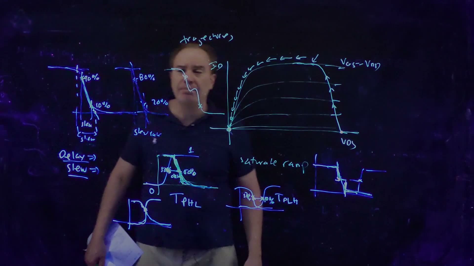
7. define the 50% delay ($t_{pHL}$tpHL​, $t_{pLH}$tpLH​) and the 10–90 and 20–80 slews, with and without extrapolation, and say where these definitions break down.

Boxes and equations marked board were written in the lecture. Parts marked added are explanations or examples this guide adds.

Before you start

You need these ideas from earlier chapters. Each is restated here.

• The three regions of an NMOS (Chapter 4). Cut off when $V_{GS} < V_T$VT​: no current. Triode when $V_{DS} < V_{GS} - V_T$VT​: the current rises steeply with $V_{DS}$VDS​. Saturated when $V_{DS} \ge V_{GS} - V_T$VT​: the current is nearly flat, almost independent of $V_{DS}$VDS​.
• PMOS signs (Chapter 4). The same rules with $V_{SG}$VSG​, $V_{SD}$ and $|V_{Tp}|$∣VTp​∣: on when $V_{SG} > |V_{Tp}|$∣VTp​∣, saturated when $V_{SD} \ge V_{SG} - |V_{Tp}|$∣VTp​∣.
• A capacitor (Chapter 0). Charge $Q = CV$CV, current $i = C\,dV/dt$CdV/dt, and stored energy $\tfrac12 CV^2$21​CV2.
• Delay is charge over current (Chapters 4 and 5). Moving the charge $CV$ with a current $I$ takes about $t = CV/I$CV/I.
• Inverters drive capacitance (Chapter 5). The output node carries the next gates’ gate capacitance plus the driver’s own drain capacitance and the wires. A PFET is made about twice as wide as the NFET ($2W$2W against $W$W) for equal drive.

Notation. $V_{Tn}$ and $V_{Tp}$ are the NFET and PFET thresholds; the lecture uses $V_{Tn} = 1\,\mathrm{V}$1V, $V_{Tp} = -1\,\mathrm{V}$ and $V_{DD} = 5\,\mathrm{V}$5V. $C_L$ is the load capacitance on the output. Exam convention added: past exams give gate capacitance per micron of width, $C_g$ in fF/µm, so a $2W/W$ inverter presents $3W\,C_g$ at its input.

1. The inverter and its transfer curve

The idea. The CMOS inverter is a PFET to the supply and an NFET to ground, driven by the same input. Its voltage transfer characteristic (VTC) is the output voltage you get for each steady input voltage.

Lecture06 @ 13:22The inverter, the two I–V families on one V_out axis (bottom left), the VTC with each region labelled, and noise rejection (right).

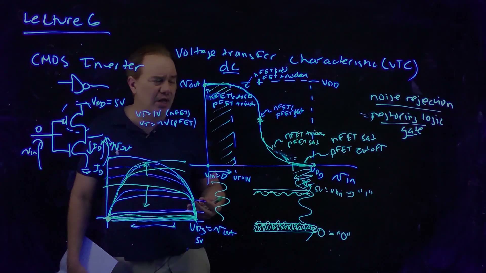
The inverter is “the quintessential digital logic gate” (00:08). Its circuit (00:17):

• a PFET from $V_{DD}$ to the output, and an NFET from the output to ground;
• both gates tied together: that is the input, $V_{in}$Vin​;
• both drains tied together: that is the output, $V_{out}$Vout​.

The VTC is a DC characteristic (00:51). Hold $V_{in}$ fixed, wait until everything settles, and read $V_{out}$Vout​. Plot $V_{out}$ against $V_{in}$Vin​; both run from 0 to $V_{DD}$VDD​.

2. Building the curve from the two I–V characteristics

The idea. In steady state the same current flows through both transistors. Draw both I–V curves against the same voltage, $V_{out}$Vout​, and the output sits where they cross.

One axis for both devices

The NFET’s drain-to-source voltage is the output: $V_{DS,n} = V_{out}$ (01:53). The PFET sits on top, and its drop is what remains of the supply: $V_{SD,p} = V_{DD} - V_{out}$Vout​, because the two drops in the stack add up to $V_{DD}$ (02:07). So the lecturer draws the PFET’s ordinary curve backwards, starting at $V_{DD}$ and running to the left (02:45). With no load drawing current at the output, the currents must match:

$$I_{D,n}(V_{in}, V_{out}) = I_{D,p}(V_{in}, V_{out}),$$

and the crossing of the two curves is the operating point.

Walking the input from 0 to the supply

The lecture uses $V_{DD} = 5\,\mathrm{V}$5V, $V_{Tn} = 1\,\mathrm{V}$ and $V_{Tp} = -1\,\mathrm{V}$ (03:57). Raise $V_{in}$ step by step:

The five regions of the VTC (board, 01:19–08:21)

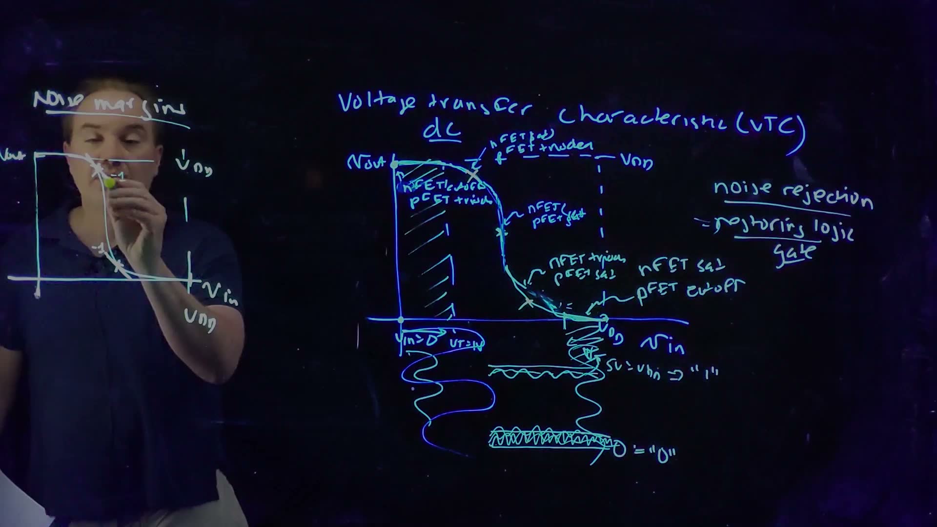
1. $V_{in} = 0$ (02:07–03:57). The NFET has $V_{GS} = 0$0: it is cut off, its curve is zero. The PFET has its full $V_{SG} = 5\,\mathrm{V}$5V. The only crossing is at $V_{out} = V_{DD}$VDD​, where the PFET carries zero current with zero $V_{SD}$VSD​: it is in triode. Output: 5 V. board “nFET cutoff, pFET triode”.
2. $V_{in}$ passes $V_{Tn} = 1\,\mathrm{V}$ (04:23–05:40). The NFET turns on and its curve starts to rise; the PFET loses overdrive and its curves come down. The output begins to drop. The NFET, with $V_{out}$ still high, is saturated; the PFET stays in triode board.
3. The middle (05:40–06:33). Eventually the curves cross where both are saturated, on their flat parts. Flat curves crossing flat curves: a tiny change in $V_{in}$ moves the crossing a long way. The output drops very fast: a region of very high gain board.
4. Past the middle (06:54–07:21). The crossing slides onto the steep part of the NFET’s curve: the NFET is in triode, the PFET saturated board.
5. $V_{in}$ above $V_{DD} - |V_{Tp}| = 4\,\mathrm{V}$ (07:21–08:21). The PFET is cut off. The NFET has full drive but no current to carry, so the crossing is at $V_{out} = 0$0: the NFET is in triode with $V_{DS} = 0$0. Output: 0 V.

A slip on the board. added The board labels the last region “nFET sat, pFET cutoff”, and the speech says “the NFET is saturated” (07:21). With $V_{DS} = V_{out} = 0$ and up to 4 V of overdrive, the NFET is in triode ($V_{DS} < V_{GS} - V_T$VDS​<VT​). The lecturer’s own words a moment later, “just the opposite of what we had over here” (07:55), point the same way: the opposite of “NFET cut off, PFET triode” is “PFET cut off, NFET triode”.

Regions along the VTCadded

$V_{in}$	NFET	PFET	$V_{out}$
$< V_{Tn}$	off	triode	$V_{DD}$
$> V_{Tn}$	sat.	triode	falls
middle	sat.	sat.	steep
past it	triode	sat.	near 0
$> 4\,\mathrm{V}$	triode	off	0

Off means cut off, sat. saturated; $4\,\mathrm{V}$ is $V_{DD} - |V_{Tp}|$ for the lecture’s numbers. NFET saturated when $V_{out} \ge V_{in} - V_{Tn}$VTn​; PFET saturated when $V_{DD} - V_{out} \ge V_{DD} - V_{in} - |V_{Tp}|$∣VTp​∣. All five regions are labelled on the board (the last one corrected, see above); the table form and the rules are added.

Holds when: steady state, no load current at the output; the NFET's V_DS is V_out and the PFET's V_SD is V_DD − V_out

Why flat curves make a steep VTC

The gain in the middle depends on how flat the saturated curves are: “the flatter these I–V characteristics, the lower the output conductance, … the steeper” the transition (06:33). If both curves were perfectly flat, the crossing would be undefined over a whole range of $V_{out}$ and the gain infinite. Real curves tilt a little, so the gain is large but finite.

Build the curve yourself. Move $V_{in}$ and watch the crossing slide; then change how strong the PFET is, and how much the saturated curves tilt.

input V_in

2.00 V

PFET strength ÷ NFET strength

1.00

output slope λ (how far the saturated curves tilt)

0.05 V⁻¹

At V_in = 2.00 V: NFET saturated, PFET triode; V_out = 4.67 V.

current through both devices

0.154 mA

gain dV_out/dV_in here

−0.90

(V_IL, V_OH)

(2.046, 4.626) V

(V_IH, V_OL)

(2.954, 0.374) V

NM_L = V_IL − V_OL

1.672 V

NM_H = V_OH − V_IH

1.672 V

largest gain (size)

30

Top: the NFET current rises with V_out and the PFET current falls; the output settles where they are equal. Bottom: that crossing traced for every V_in. The shaded band is where the gain is larger than 1 in size; the dashed segments have slope −1. The devices follow Chapter 4's long-channel (square-law) model with the saturated curves tilted by (1 + λV_DS), at the lecture's V_DD = 5 V and V_T = ±1 V; the strengths are illustrative. The lecture draws the curves without a model, so read the shapes, not the decimals. PFET ÷ NFET strength = 1.00 means β_p = 1.00 β_n.

What to notice.

• Sweep $V_{in}$ slowly from 0. Nothing happens until 1 V, then the output falls a little, then all at once around 2.5 V, then it settles at 0 by 4 V. The region banner walks through the five rows of the table.
• With equal strengths the curve is symmetric and switches at $V_{DD}/2 = 2.5\,\mathrm{V}$2.5V.
• Make the PFET stronger: the NFET has to be pushed harder before it can win, so the whole curve moves right. Make it weaker and the curve moves left. added The lecture doesn’t discuss sizing; this follows from its crossing construction.
• Tilt the saturated curves more (raise λ): the middle gets less steep and the largest gain falls. This is the lecture’s “lower output conductance, steeper” point, run backwards.

Check yourself At V_in = 3 V in the lecture's inverter (V_DD = 5 V, V_T = ±1 V), the output has settled at about 0.3 V. Which region is each transistor in?

NFET: $V_{GS} - V_{Tn} = 2\,\mathrm{V}$ and $V_{DS} = 0.3\,\mathrm{V} < 2\,\mathrm{V}$2V, so triode. PFET: $V_{SG} - |V_{Tp}| = 2 - 1 = 1\,\mathrm{V}$ and $V_{SD} = 4.7\,\mathrm{V} \ge 1\,\mathrm{V}$1V, so saturated. This is the “past the middle” row.

3. Noise rejection: a restoring logic gate

The idea. The curve is flat near both ends. A noisy input near 0 or near $V_{DD}$ therefore produces an almost noise-free output: the inverter restores clean logic levels.

Why “inverter”. We let voltages near 0 stand for logic 0 and voltages near $V_{DD}$ for logic 1 (08:21). Low inputs give high outputs and high inputs give low outputs, so the circuit computes the Boolean NOT.

The shape is the point (08:55–09:49). Used as an amplifier, you would bias the inverter in its steep middle, where the small-signal gain is huge. But for logic, what matters is what that steep middle does to the ends: it makes them flat. The property is called noise rejection, and a gate with it is a restoring logic gate board.

Noise is always there (10:22–11:15). A logic 0 is never exactly 0 V. Coupling from neighbouring wires, variations in the power supply and interference all disturb node voltages. The noise may be DC (the level sits a little above ground, or a little below $V_{DD}$VDD​) or AC (it wiggles).

How the inverter cleans it (11:15–12:00). Put a noisy logic 0 at the input. The VTC is nearly flat there, so the output hardly moves: the noise is suppressed. The same happens around $V_{DD}$VDD​. Every gate hands the next one a cleaner signal than it received. The lecturer calls this “absolutely essential” and “the fundamental strength of digital gates” (12:09).

A cautionary tale (12:43–14:14). In the 1970s IBM tried to build a computer from superconducting Josephson junctions, cooled to about 4 K. The project failed. The cooling was a nuisance, but the lecturer’s point is the real reason: those gates did not have a transfer curve like this, so they could not reject the coupling noise that grew as the circuits were scaled down. CMOS can, and “that’s why it’s basically taken over the world.”

Check yourself Why does a flat VTC near 0 V reject noise, while a steep one would amplify it?

The output change is the input change times the slope, $dV_{out}/dV_{in}$dVout​/dVin​. Where the curve is flat the slope is near 0, so input noise barely reaches the output. Where it is steep, the slope is larger than 1 in size and the noise comes out bigger than it went in.

4. Noise margins

The idea. Noise rejection has a limit. If the noise is big enough to push an input into the steep part, the gate amplifies it. The noise margins say how much noise each logic level can take before that happens.

Lecture06 @ 24:16Noise margins: the −1 points (left), the two assumptions (top), the chain with a noise source on every node, NM_L and NM_H, and the low-pass remark (bottom left).

The two points of slope −1

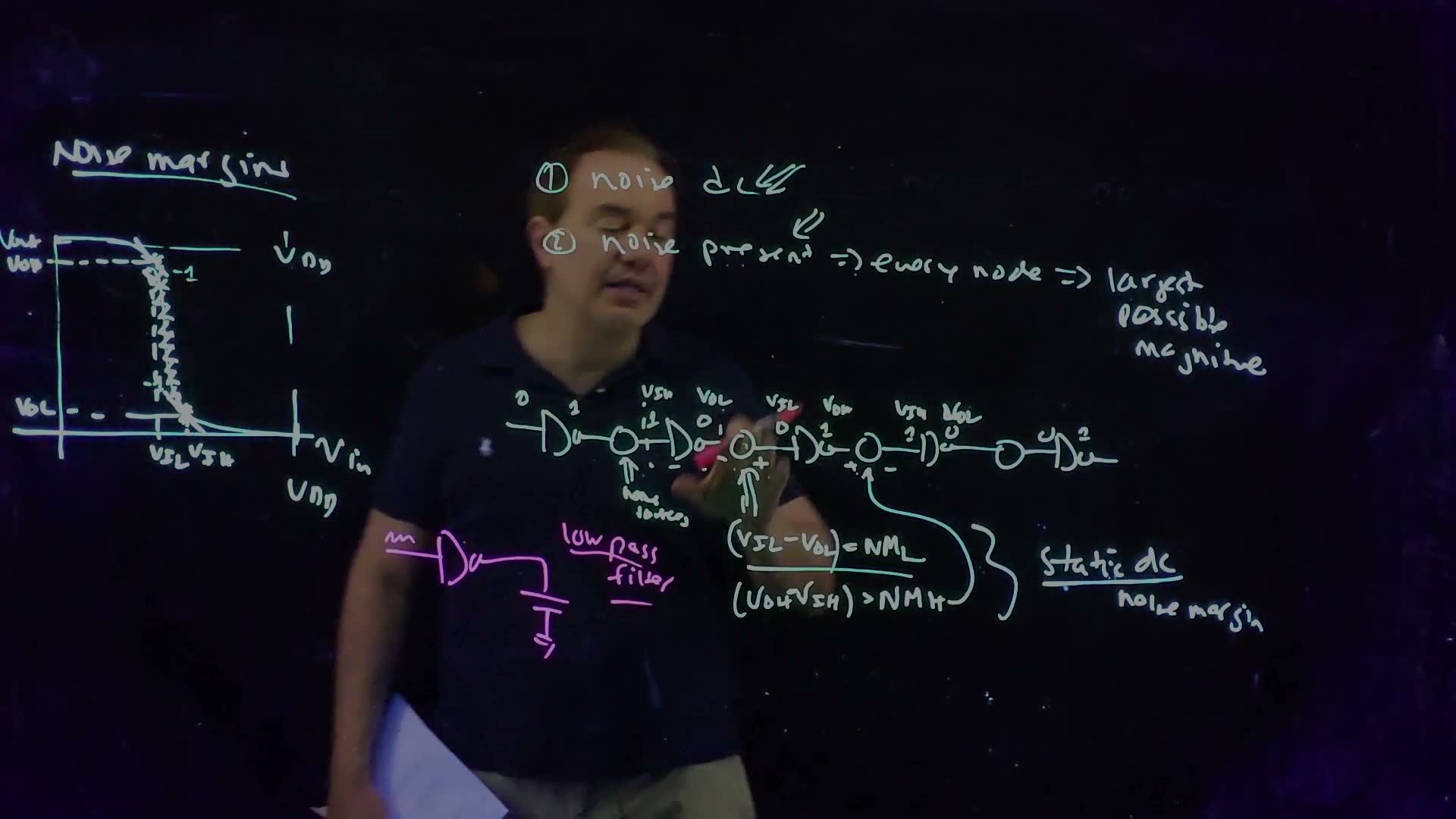
Mark the two points on the VTC where the slope is exactly −1 (15:58):

• between them the gain is larger than 1 in size: a “no man’s land” where noise is amplified (16:41);
• outside them the gain is smaller than 1: noise is rejected.

The coordinates of these points get names (16:58) board:

• the upper point is $(V_{IL}, V_{OH})$(VIL​,VOH​): V input low, V output high;
• the lower point is $(V_{IH}, V_{OL})$(VIH​,VOL​): V input high, V output low.

So an input below $V_{IL}$ is safely a 0, an input above $V_{IH}$ safely a 1, and a good gate’s outputs are at least $V_{OH}$ (high) and at most $V_{OL}$ (low).

Two conservative assumptions

To define the margins, the lecture makes two deliberately pessimistic assumptions (17:15–18:25) board:

1. the noise is DC;
2. the noise is present on every node, with the largest possible magnitude.

Picture a long chain of inverters with a DC noise source in series between each pair (18:25). With the largest possible noise everywhere, every inverter is pushed right to the edge: each one sits exactly at one of the −1 points, “on the hairy edge of amplifying noise” (20:05). Down the chain they alternate: input $V_{IH}$ with output $V_{OL}$VOL​, then input $V_{IL}$ with output $V_{OH}$VOH​, and so on.

The noise margins (board, 20:25–21:23)

1. Take a node that should be low. The inverter driving it is at its worst, so the node already sits at $V_{OL}$VOL​.
2. The next inverter starts to amplify when its input reaches $V_{IL}$VIL​. So the noise source on that node can add at most $V_{IL} - V_{OL}$ board. That is the noise margin low, $NM_L$NML​.
3. Take a node that should be high. Its driver leaves it at $V_{OH}$VOH​, and the next inverter amplifies once its input drops to $V_{IH}$VIH​. The noise can take away at most $V_{OH} - V_{IH}$ board: the noise margin high, $NM_H$NMH​.

Static DC noise marginsboard

$$NM_L = V_{IL} - V_{OL}$$$$NM_H = V_{OH} - V_{IH}$$

$NM_L$ is how much DC noise a low node can take (pushing it up); $NM_H$ how much a high node can take (pulling it down).

Holds when: DC noise on every node, each at its largest possible value; V_IL, V_OH, V_IH, V_OL at the two slope −1 points of the VTC

The widget in Section 2 marks both −1 points, shades the band between them and reads out both margins.

Worked example. added The widget’s default inverter: the lecture’s 5 V and ±1 V, equal strengths. The numbers come from that model’s curve; the lecture draws the curve but gives no values.

1. Read the upper −1 point: $V_{IL} = 2.046\,\mathrm{V}$2.046V, $V_{OH} = 4.626\,\mathrm{V}$4.626V.
2. Read the lower −1 point: $V_{IH} = 2.954\,\mathrm{V}$2.954V, $V_{OL} = 0.374\,\mathrm{V}$0.374V.
3. $NM_L = V_{IL} - V_{OL} = 2.046 - 0.374 = 1.672\,\mathrm{V}$1.672V.
4. $NM_H = V_{OH} - V_{IH} = 4.626 - 2.954 = 1.672\,\mathrm{V}$1.672V. Equal, because this inverter is symmetric.
5. Make the PFET twice as strong (slider to 2.00): the curve moves right. Now $V_{IL} = 2.389$2.389, $V_{OH} = 4.587$4.587, $V_{IH} = 3.282$3.282, $V_{OL} = 0.294\,\mathrm{V}$0.294V, so $NM_L = 2.389 - 0.294 = 2.095\,\mathrm{V}$ grows and $NM_H = 4.587 - 3.282 = 1.305\,\mathrm{V}$ shrinks. (The widget’s third decimal can differ by one, from rounding.)

Common mistakes.

• Swapping the pairs. $V_{IL}$ goes with $V_{OH}$ (the same point), but $NM_L$ pairs $V_{IL}$ with $V_{OL}$ (from different points). Each margin compares what one gate outputs with what the next gate accepts.
• Using the switching point (where $V_{out} = V_{in}$Vin​) as the limit. The limit is where the slope reaches −1, well before the middle.

Check yourself Three inverters have W_p/W_n = 1/1, 2/1 and 4/1 µm. Their VTCs switch at three different inputs. Which curve is which, and which gives the largest NM_H?

A stronger PFET moves the curve right, so from left to right the curves are 1/1, 2/1, 4/1. $NM_H = V_{OH} - V_{IH}$VIH​, and $V_{OH}$ hardly changes, so the largest $NM_H$ belongs to the smallest $V_{IH}$VIH​: the left-most curve, 1/1. (This is MT17-2; the widget shows the same trend.)

Check yourself With technology scaling the inverter's largest gain falls (the saturated curves tilt more). What happens to V_IL, V_IH and the two noise margins?

A less steep middle means the −1 points spread apart: $V_{IL}$ moves down and $V_{IH}$ moves up. Both margins shrink. Try it with the λ slider: from 0.05 to 0.2 V⁻¹ both margins fall from 1.67 V to 1.52 V. (MT24-1d asks this; how $V_{OH}$ and $V_{OL}$ move depends on the device model.)

5. Why the textbook margins are conservative

The idea. Both assumptions are worst cases. Real noise is rarely on every node at full size, and rarely DC, so real gates tolerate more than $NM_L$ and $NM_H$NMH​.

Every node, largest magnitude (21:29–22:31). The margin $V_{IL} - V_{OL}$ is small because the previous node is also noisy: its output was already pushed to $V_{OL}$VOL​. If that node were clean, it would sit at ground, and the noise source could push this node all the way up to $V_{IL}$ before the next gate amplified. On the high side the same reasoning gives $V_{DD} - V_{IH}$VIH​. (“There’s also no noise here” at 22:31 is a slip: the board’s point is that there is noise on the previous node.)

If only one node is noisyadded

$$\text{low node: up to } V_{IL}$$$$\text{high node: a drop of } V_{DD} - V_{IH}$$

Holds when: DC noise on a single node; the gate driving it has a clean input, so its output is at the rail (spoken at 21:29–22:31, not on the board)

These are larger than $NM_L$ and $NM_H$NMH​. The board calls the every-node version the static DC noise margins (22:59), “the textbook definition”, and the lecturer notes the redundancy (“static implies DC”).

DC is the worst kind of noise (23:27–24:53). An inverter driving a load capacitance has a delay; in other words it acts as a low-pass filter board. Short AC noise is filtered out before it can flip the output, so the margins for AC noise are better than the DC ones. “These textbook definitions of noise margins are extremely conservative on at least two accounts.” added The low-pass argument helps, but a DC margin is not a guarantee against every short glitch; a large enough pulse still gets through.

Worked example. added The default inverter of Section 4. A low node in a chain where every node is noisy can take $NM_L = 1.672\,\mathrm{V}$1.672V; if it is the only noisy node it can take $V_{IL} = 2.046\,\mathrm{V}$2.046V. A high node: $NM_H = 1.672\,\mathrm{V}$ against $V_{DD} - V_{IH} = 5 - 2.954 = 2.046\,\mathrm{V}$2.046V.

Check yourself Does the fanout of a CMOS gate (how many gates its output drives) change its static DC noise margins?

No. The static DC margins come from the DC transfer curve. Extra fanout adds capacitance to the output, which changes how fast the gate switches but not where the settled output is for a given input: a capacitor carries no DC current. (This is MT17-1a.)

Check yourself In MT24-1 the noise is first on every node, then on only one node. For each case, how much DC noise can a low node take, and a high node?

Every node: $NM_L = V_{IL} - V_{OL}$ on a low node and $NM_H = V_{OH} - V_{IH}$ on a high node. One node only: $V_{IL}$ on a low node and $V_{DD} - V_{IH}$ on a high node, because the gate driving it outputs a clean 0 V or $V_{DD}$VDD​.

6. Switching energy

The idea. Charging a capacitor to $V_{DD}$ from a fixed supply always takes $C_LV_{DD}^2$ from the supply. Half ends up stored on the capacitor, half is burnt as heat on the way, and the stored half is burnt when the capacitor is discharged.

Lecture06 @ 31:28The switching-energy derivation: E = C_L V_DD² from the supply (boxed, right), ½ C_L V_DD² stored (boxed, left).

Energy drawn from the supply

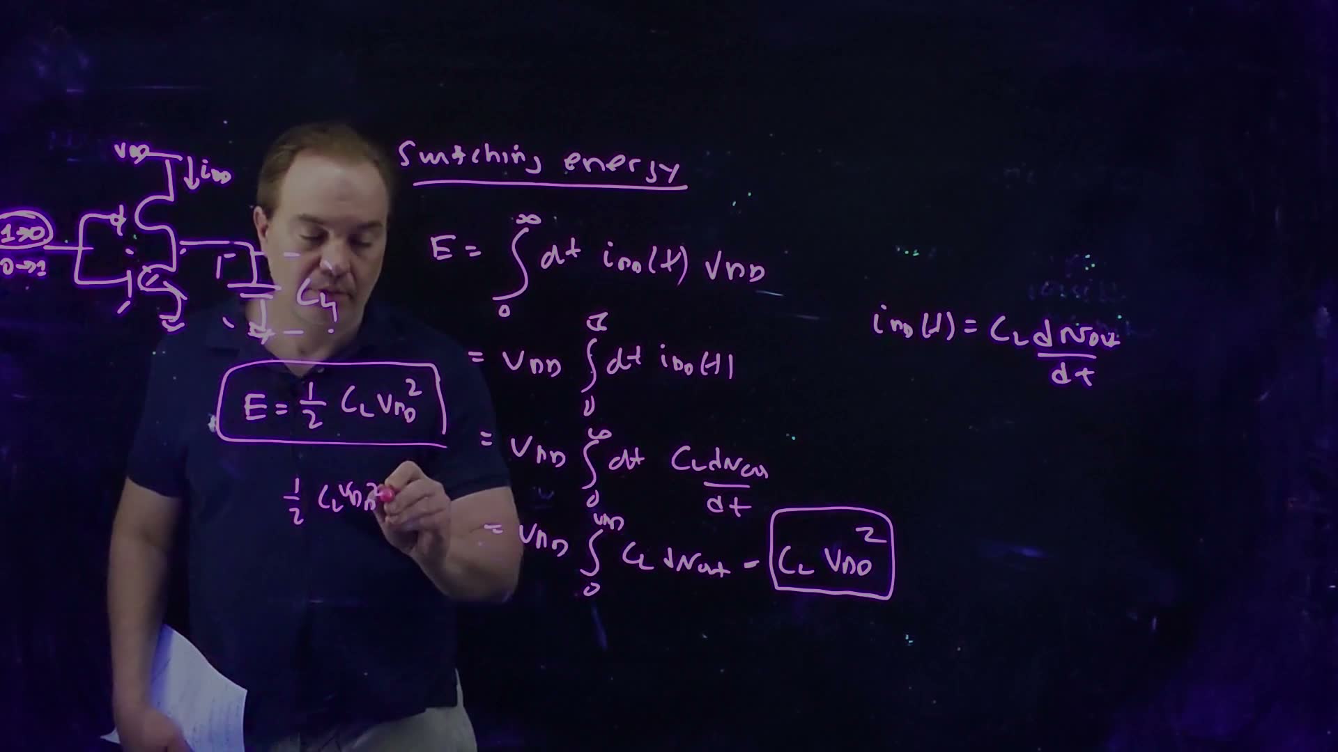
Take the inverter driving a load $C_L$ (26:08). The load is whatever hangs on the output: wires, and the gates of the next stages. Switch the input from 1 to 0: the PFET turns on and charges $C_L$ to $V_{DD}$VDD​. Switch it back to 0 → 1 and the NFET discharges it. Where does the energy come from, and where does it go?

All of it comes out of the supply (27:34): a current $i_{DD}$ flows out of $V_{DD}$VDD​.

Energy from the supply while charging (board, 27:58–29:27)

1. Power from a fixed supply is $V_{DD}\,i_{DD}(t)$VDD​iDD​(t), so over the whole transient board: $E = \displaystyle\int_0^\infty i_{DD}(t)\,V_{DD}\,dt$∫0∞​iDD​(t)VDD​dt.
2. $V_{DD}$ is constant; take it out board: $E = V_{DD}\displaystyle\int_0^\infty i_{DD}(t)\,dt$VDD​∫0∞​iDD​(t)dt.
3. With the NFET off, all the supply current charges the capacitor board: $i_{DD}(t) = C_L\,\dfrac{dV_{out}}{dt}$CL​dtdVout​​.
4. Substitute: $E = V_{DD}\displaystyle\int_0^\infty C_L\,\dfrac{dV_{out}}{dt}\,dt$VDD​∫0∞​CL​dtdVout​​dt.
5. Change the variable to $V_{out}$ added: $\dfrac{dV_{out}}{dt}\,dt = dV_{out}$dVout​, and $V_{out}$ goes from 0 to $V_{DD}$VDD​.
6. $E = V_{DD}\displaystyle\int_0^{V_{DD}} C_L\,dV_{out} = C_LV_{DD}^2$ board.

Where it goes

The energy stored on a charged capacitor is $\tfrac12 C_LV_{DD}^2$ (29:48), “from your circuits 101 class”. So charging took $C_LV_{DD}^2$ out of the supply and stored only half of it. “Where did the other half go?” (30:24)

In a circuit, energy can only be stored (on capacitors or inductors), dissipated as heat, or radiated, as an antenna does (30:30). A phone’s battery energy goes to radiation and heat. Here nothing radiates, so the other half became heat, in the PFET that carried the current (31:11).

Then switch the input back (31:32). The capacitor discharges through the NFET (the speech says “through the inductor”: a slip) and its stored half is dissipated as heat too. Nothing is drawn from the supply during the discharge. So every full cycle, charge then discharge, burns $C_LV_{DD}^2$CL​VDD2​.

Switching energy and dynamic powerboard

$$E_{\text{supply}} = C_LV_{DD}^2 \ \text{per charge}$$$$E_{\text{stored}} = \tfrac12 C_LV_{DD}^2$$$$P = C_LV_{DD}^2\,f$$

Charging: $\tfrac12 C_LV_{DD}^2$ stored, $\tfrac12 C_LV_{DD}^2$ heat. Discharging: the stored half becomes heat. This is the dynamic power (33:18).

Holds when: fixed supply, constant C_L, full swing 0 ↔ V_DD; no crowbar or leakage current; f counts full charge–discharge cycles

It doesn’t depend on the waveform (32:58). Nothing in the derivation used the shape of $V_{out}(t)$ or the transistor’s I–V curve. A weak or strong PFET, a fast or slow edge: the supply always delivers $C_LV_{DD}^2$ per charge. “This is a fundamental property of charging a capacitor.”

See it below. The charging path is drawn as a plain resistor; change it, and only the timing changes.

load C_L

20 fF

supply V_DD

1.2 V

resistance of the charging path R

2.0 kΩ

switching frequency f (full cycles)

1.0 GHz

from the supply while charging, C_LV_DD²

28.8 fJ

stored on C_L, ½C_LV_DD²

14.4 fJ

heat while charging (pull-up)

14.4 fJ

heat while discharging (pull-down)

14.4 fJ

per full cycle

28.8 fJ

power C_LV_DD²f

28.8 µW

time constant RC_L

40 ps

Change R: the waveform gets faster or slower, but the energies end at the same values. The supply only gives energy while it charges the node (the red supply curve is flat during the discharge). The pull-up and pull-down are drawn here as a plain resistor R; the lecture's result needs no device model, so a transistor gives the same totals. The input switches at 0 and at 1000 ps; with the largest R and C_L the node is still less than 1% short of the rail when it switches back; the readouts give the settled values.

What to notice.

• During charging the red curve (supply) climbs to $C_LV_{DD}^2$ while the stored and heat curves each climb to half of it, at every R.
• During discharge the red curve stays flat, the stored energy falls to zero, and the heat rises to $C_LV_{DD}^2$CL​VDD2​.
• Doubling $V_{DD}$ quadruples the energy: the square is why lowering the supply saves so much power.

Energy in a chain of gates

Worked example. added A chain of four $2W/W$ inverters with $W = 2\,\mu\mathrm{m}$2μm, in the exam conventions: $C_g = 1.5\,\mathrm{fF/\mu m}$1.5fF/μm, 3 fF of wire on every output, and the last output loaded by one more inverter input. Ignore drain capacitance. $V_{DD} = 1\,\mathrm{V}$1V.

1. Every output carries one inverter input plus wire: $C = 3W\,C_g + 3\,\mathrm{fF} = 3(2)(1.5) + 3 = 12\,\mathrm{fF}$12fF.
2. The input rises once. Outputs 1 and 3 fall; outputs 2 and 4 rise.
3. Only the rising nodes draw from the supply: $E_{\text{supply}} = 2 \times C_LV_{DD}^2 = 2 \times 12\,\mathrm{fF} \times 1^2 = 24\,\mathrm{fJ}$24fJ.
4. Energy dissipated in this one transition: the two charging nodes burn half of their 12 fJ each, and the two discharging nodes burn their stored 6 fJ each: $4 \times 6 = 24\,\mathrm{fJ}$24fJ. The same number, by a different count.
5. A full input cycle (up, then down) charges every node once: $4 \times 12 = 48\,\mathrm{fJ}$ from the supply.
6. At one input cycle per nanosecond, $f = 1\,\mathrm{GHz}$1GHz: $P = 48\,\mathrm{fJ} \times 10^9\,\mathrm{s^{-1}} = 48\,\mu\mathrm{W}$48μW.

Leakage energy uses the same integral. added If a transistor that is off still leaks a steady current $I_{leak}$ (Chapter 4’s subthreshold current), step 1 of the derivation gives $E = V_{DD}I_{leak}T$ over a time $T$T. For example, if each of the four inverters leaks 1 µA, in one 1 ns cycle the chain leaks $4 \times 1\,\mu\mathrm{A} \times 1\,\mathrm{V} \times 1\,\mathrm{ns} = 4\,\mathrm{fJ}$4fJ, which is $4/(48 + 4) = 7.7\%$ of the total.

Common mistakes.

• Counting $C_LV_{DD}^2$ for every node that switches. Per transition, only the nodes that rise draw from the supply.
• Mixing up “drawn from the supply” and “dissipated”. Over a full cycle both are $C_LV_{DD}^2$ per node; within one transition they are counted differently, as steps 3 and 4 show.
• Using $f$ as the number of edges. $P = C_LV_{DD}^2f$ counts full charge-and-discharge cycles; counting both edges doubles the power.
• Thinking a slower (more resistive) pull-up wastes less. The heat is $\tfrac12 C_LV_{DD}^2$ whatever the resistance.

Check yourself A node of 20 fF switches between 0 and 1.2 V. How much energy does one rising edge draw from the supply, how much is stored, and how much does a full cycle burn?

From the supply: $C_LV_{DD}^2 = 20\,\mathrm{fF} \times 1.44\,\mathrm{V^2} = 28.8\,\mathrm{fJ}$28.8fJ. Stored: half, 14.4 fJ. A full cycle burns all of it, 28.8 fJ (14.4 fJ while charging, 14.4 fJ while discharging).

Check yourself A chain of N identical inverters is driven by a square wave of period T. Each output carries C. How much energy does the chain draw from the supply per period, ignoring crowbar and leakage?

In one period every output rises exactly once, so the chain draws $N\,C\,V_{DD}^2$NCVDD2​. (MT23-1a and MT24-2a ask this, with $C = 3W\,C_g$ plus a side load for 2W/W inverters, or $2W\,C_g$ plus the side load for W/W ones.)

7. Crowbar current and slew

The idea. While the input is between the thresholds, both transistors are on, and some current flows straight from $V_{DD}$ to ground without charging anything. The slower the input changes, the longer this lasts.

Lecture06 @ 37:20Crowbar current (left), 'wasted' power at 10–20% of the dynamic power, and Power = C_L V_DD² f (right).

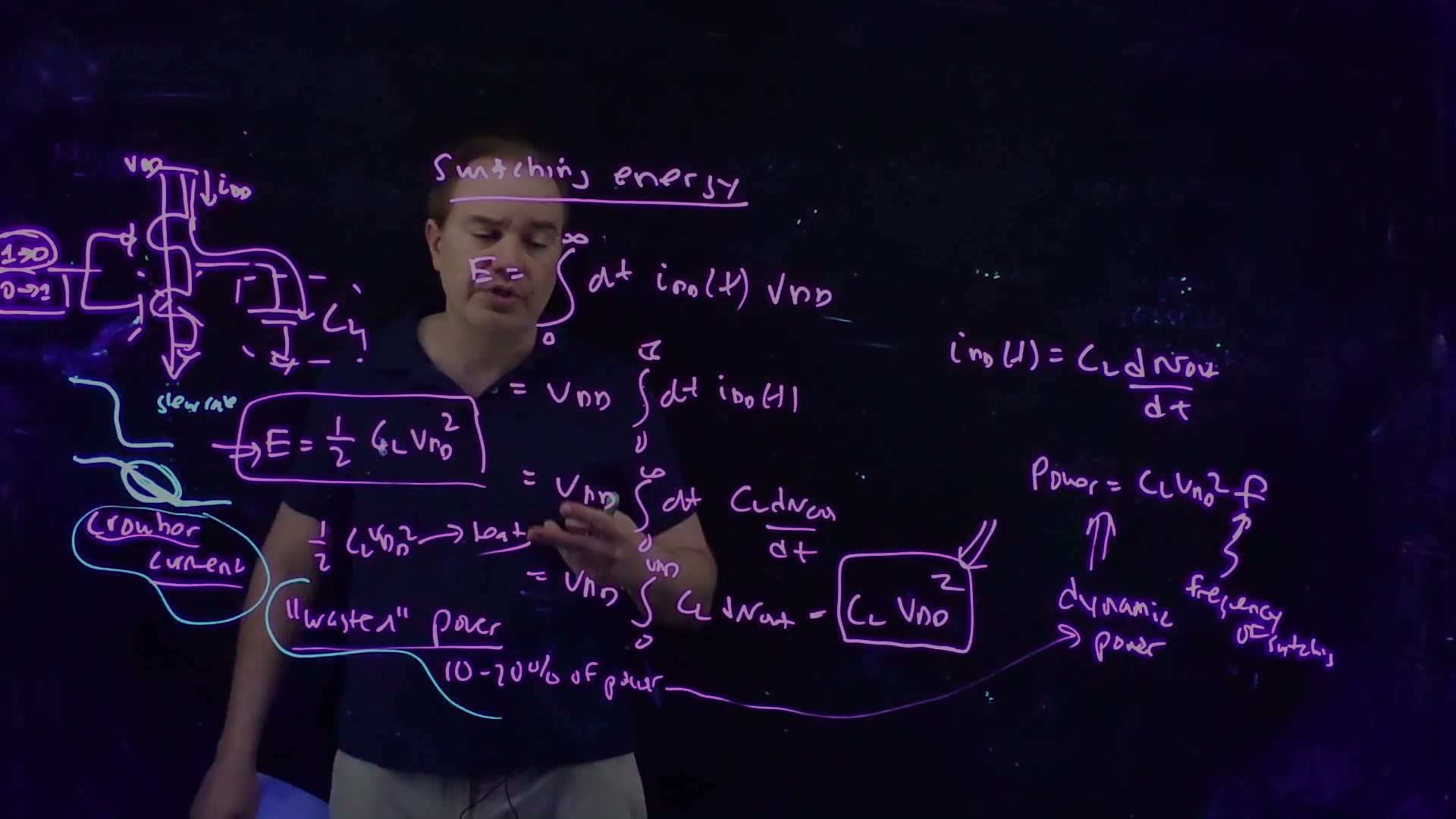
The energy derivation assumed all the supply current charged the capacitor (33:51). In reality, during the transition there is a period when both devices are on (34:10), as the VTC’s middle regions showed. Current then flows directly from $V_{DD}$ to ground: the crowbar current board. Its energy does nothing useful, so it is part of the “wasted” power.

• Typically it costs about 10–20% of the dynamic power (35:09) board. That is the lecturer’s figure for most designs, not a law.
• A fast input edge minimises it; a slow one leaves both devices on longer and makes it worse (35:35).
• How fast a signal changes from 0 to 1 is its slew rate (36:12). Designs set a slew-rate target for every node: no node may slew more slowly than a set limit (36:44).
• There are two reasons: crowbar power, and noise. A slowly changing node spends a long time near the steep middle of the next gate’s VTC, where it picks up noise easily (37:00).
• Slow nodes have a nickname: dog nodes, “as in slow as a dog” (37:16).

The widget in Section 9 measures the crowbar energy of one edge. With its default inverter and a 50 fF load, a 100 ps input edge wastes 0.4% of $C_LV_{DD}^2$CL​VDD2​, a 500 ps edge 5.6%.

Check yourself Why does making the input edge faster reduce crowbar energy, while it does nothing to the C_LV_DD² switching energy?

The crowbar current flows only while the input is between $V_{Tn}$ and $V_{DD} - |V_{Tp}|$∣VTp​∣, when both devices conduct; a faster edge shortens that window. The switching energy is fixed by the charge $C_LV_{DD}$ delivered at $V_{DD}$VDD​, whatever the waveform.

8. Compact models, variability and process corners

The idea. Simulators use heavily parameterised transistor models. Every parameter varies from device to device, so designers simulate at extreme but consistent settings, the corners, to make sure the chip still works.

Lecture06 @ 50:12Compact models, variability, the five corners (TT, SS, FF, SF, FS) and PVT.

Compact models

The transistor models used in circuit simulation are compact models, also called SPICE models after SPICE, the first circuit simulator, written at Berkeley (38:37) board. The most widely used family is BSIM (38:59); the lecturer is unsure whether it is up to BSIM5 or BSIM6. These models have very many parameters. They began as physics-based models but have become “glorified curve fits” (39:42). You will load such model files in the CAD tools.

Variability

No two transistors are identical (40:27):

• each parameter, such as the channel length $L$ or the threshold $V_T$VT​, follows a distribution around its nominal value board;
• parameters can be correlated, for example $V_T$ with $L$L, and the models capture that (41:12);
• variation happens at every scale: within a die, across the reticle, across a wafer, and from wafer to wafer (41:43).

Corner models

The most conservative approach lumps every source of variation together and pushes everything to the edge at once (42:09). These are corner models, usually three-sigma models: each parameter set three standard deviations from its mean (42:35) board. Each corner is named by two letters, the NFET’s then the PFET’s (42:49):

Corner	Meaning	Use
TT	typical NFET, typical PFET: every parameter nominal; the simulator’s default (43:14)	normal design
SS	slow–slow: $\lvert V_T\rvert$ and $L$ at their largest, less overdrive (45:33)	check the clock frequency: does the chip still meet timing? (46:28)
FF	fast–fast: the other direction, $\lvert V_T\rvert$ low, $L$ short (47:10)	the fast extreme
SF, FS	slow NFET with fast PFET, and the reverse: the skewed corners (47:25)	circuits sensitive to the NFET-to-PFET strength ratio (48:38)

A common misconception (47:45–48:38). The slow NFET of the SF corner is not as slow as the SS NFET, and its fast PFET not as fast as the FF PFET. Both devices sit on the same chip, so SF is “the maximum amount the P and the N can be different from each other in opposite directions”, which is less extreme than mixing the two other corners. added The letter order (NFET first) is how the lecture says it; check the model documentation of any real process before relying on it.

Yield and PVT

All of this serves yield: the fraction of manufactured chips that work (43:44). Chips that fail are thrown away, or, as the lecturer recalls, sold by Intel as ten-dollar Christmas-tree ornaments instead of thousand-dollar processors. “Yield is money.”

To maximise yield, a circuit must work across PVT variation (48:57) board:

• process: the corners above;
• voltage: supply noise and variation; a lower supply is slower, so a timing check pairs the SS corner with the lowest supply (49:53);
• temperature: a hotter chip is slower, and it also leaks more (50:20).

Check yourself You must show that a chip meets its clock frequency. Which corner and which supply voltage do you simulate, and why?

The slow–slow (SS) corner at the lowest supply voltage the chip may see, and hot. All three make the transistors as slow as they can be, so if the timing passes there, it passes everywhere in the PVT range.

Check yourself Why isn't the SF corner simply the SS corner's NFET combined with the FF corner's PFET?

Because the two devices are made together on one chip. Their parameters can’t both sit at opposite three-sigma extremes at once; SF is the largest difference between the NFET and the PFET, which is smaller than combining two separate extremes.

9. Delay: trajectories and the saturated ramp

The idea. When an inverter discharges its load, its NFET’s operating point traces a path, a trajectory, across the I–V curves: up to full drive, along the flat part at nearly constant current, then down through triode as the output nears zero.

Lecture06 @ 55:58The NFET's trajectory as it discharges C_L (centre), the real output waveform (left) and its saturated-ramp abstraction (right).

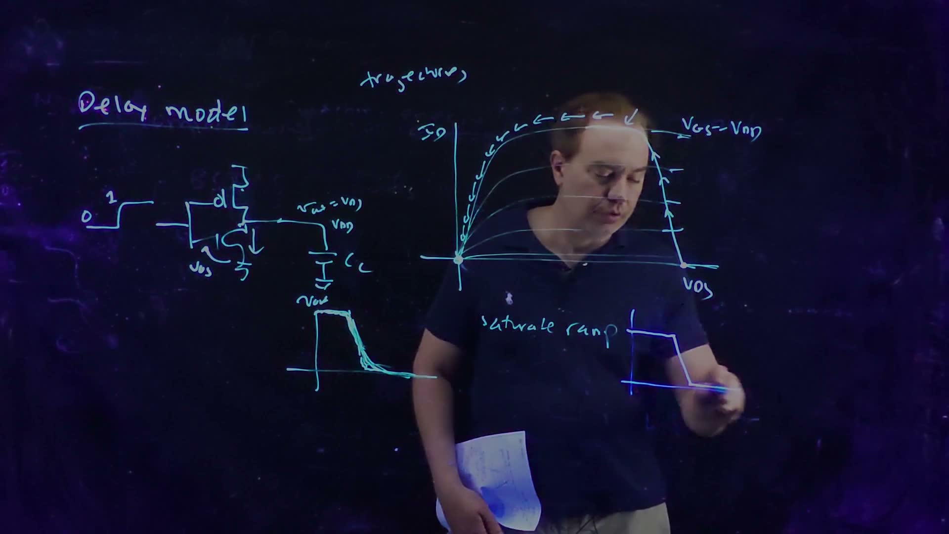
Follow one edge (51:52–54:51): the input goes from 0 to 1, the output starts at $V_{DD}$VDD​, and the NFET discharges $C_L$CL​.

1. Up. At first $V_{out} = V_{DD}$ and the input is rising, so the operating point climbs straight up the right edge of the I–V plane, from one $V_{GS}$ curve to the next, until it reaches the $V_{GS} = V_{DD}$ curve. How fast it climbs depends on the input’s slew (53:39).
2. Along. Now the NFET is saturated with full overdrive. It removes charge at a nearly constant current, so $V_{out}$ falls along a nearly straight line (54:07).
3. Down. As $V_{out}$ falls below the overdrive, the NFET enters triode. Its current shrinks with $V_{DS}$VDS​, so the output approaches zero slowly, along a long, roughly exponential tail: the device acts more like a resistor (54:51).

The saturated ramp (55:21). Real waveforms have curved starts and long tails. Designers abstract each one as a saturated ramp: flat, a straight ramp, flat again. (The lecturer says “saturate ramp”.) Delay and slew are the two numbers that describe such a ramp.

Edge:Input rises (t_pHL)Input falls (t_pLH)

input slew (0 → V_DD ramp time)

100 ps

load C_L

50 fF

PFET strength ÷ NFET strength

1.00

delay t_pHL (50% to 50%)

78.1 ps

output 10–90% time

140 ps

extrapolated 10–90 slew

175 ps

output 20–80% time

87.9 ps

extrapolated 20–80 slew

146 ps

energy from the supply, this edge

4.9 fJ

crowbar part

4.9 fJ = 0.4% of C_LV_DD²

Top: the dots mark where the input and the output cross 50% of V_DD; the delay is the time between them, and it can come out negative. Bottom: the current of the device that switches the output, against V_out. A fast input puts it on the full-drive curve at once; a slow one climbs up while the output is already moving. Square-law devices at V_DD = 5 V and V_T = ±1 V, as in the transfer-curve widget, integrated numerically; the numbers are illustrative, the shapes are the point.

What to notice.

• With a fast input (10–50 ps) the trajectory jumps up to the full-drive curve and rides it down, exactly the board’s picture. Slow the input down and the trajectory climbs gradually while the output is already falling; it never reaches the full-drive curve.
• More load stretches the output ramp; the input slew stretches it less.
• The crowbar readout grows quickly with the input slew (Section 7).

10. Defining delay and slew

The idea. Delay is measured between the 50% points of the input and output. Slew is the duration of one transition, but there are several conventions for measuring it, so always ask which one is meant.

Lecture06 @ 63:14Delay from 50% to 50% (t_pHL, t_pLH), the 10–90 and 20–80 slews with and without extrapolation, and the ill-behaved waveforms.

Delay: 50% to 50%

Take the time at which the input crosses 50% of its swing and the time at which the output crosses 50% of its swing (56:35). The difference is the delay, or propagation time board:

• $t_{pHL}$tpHL​: the output goes high to low (input rising);
• $t_{pLH}$tpLH​: the output goes low to high (input falling).

Everything else, the tails and the curvature, is ignored (57:51). “This is the almost universal definition of delay.”

A constant-current estimate. added If the switching device delivered a constant current $I$I, the output would fall linearly, and reaching 50% means removing half the charge: $t_p \approx C_L(V_{DD}/2)/I = C_LV_{DD}/(2I)$CL​VDD​/(2I). This is Chapter 5’s $t = CV/I$ taken to the 50% point. For example, 20 fF at 1 V with 100 µA gives $20\,\mathrm{fF} \times 1\,\mathrm{V}/(2 \times 100\,\mu\mathrm{A}) = 100\,\mathrm{ps}$100ps.

A weakness: negative delay

The 50% definition can give negative delays (57:59–59:31). It doesn’t happen often, and only when “weird stuff” is going on, typically with a poorly sized gate that cannot drive its load, so its output slews very slowly. That slow signal is the next gate’s input. If that next gate is strong and lightly loaded, its own output can swing past 50% before its slowly rising input reaches 50%. The output is still responding to the input, just to its early part. added The speech pairs “a very fast switching input” with “a very slowly slewing output”; the arrangement that actually gives a negative 50% delay is a slow input with a fast output, as above.

Try it in the widget: choose Input falls, set the input slew to 1000 ps, the load to 10 fF and the PFET strength to 4. The rising output crosses 50% about 51 ps before the input does. The lecturer’s verdict: “this is more a statement of the weakness of this kind of a metric … but it is what everyone uses” (58:56).

Slew: no single definition

On a perfect saturated ramp, the slew is simply the ramp’s duration (60:20). Real waveforms have tails, so the conventions measure between points that avoid them (60:46–61:50) board:

• 10–90 slew: the time between the 10% and 90% points;
• extrapolated 10–90 slew: draw the line through those two points and extend it to $V_{DD}$ and to ground; take the time between those crossings. This is closer to the saturated ramp, and “more commonly done”;
• 20–80 slew, and extrapolated 20–80 slew, the same with the 20% and 80% points.

For a straight ramp the extrapolations agree. added The 10% and 90% points are 80% of the swing apart, so the extrapolated slew is the 10–90 time divided by 0.8; for 20–80 divide by 0.6. A ramp that takes 100 ps from rail to rail has a 10–90 time of 80 ps and a 20–80 time of 60 ps, and both extrapolate back to 100 ps. On a curved waveform the two extrapolations differ.

Delay and slewboard

$$t_{pHL},\ t_{pLH} = t_{out,50\%} - t_{in,50\%}$$$$\text{slew}_{10\text{–}90} = |t_{90\%} - t_{10\%}|$$$$\text{slew}_{20\text{–}80} = |t_{80\%} - t_{20\%}|$$$$\text{extrapolated: } \frac{\text{slew}_{10\text{–}90}}{0.8}, \quad \frac{\text{slew}_{20\text{–}80}}{0.6}$$

Holds when: input and output swing rail to rail; the slew formulas in the last line assume the straight-line extrapolation (added)

Buyer beware (61:50). “There is really no standard.” Whenever someone quotes a slew rate, ask: 10–90 or 20–80? Extrapolated or not?

When the abstraction fails (62:18–63:23). Coupling noise can put bumps in a waveform. What is the delay or the slew of a signal that crosses 50% three times? The formulas still give numbers, but they no longer describe the waveform. Digital design simplifies analog waveforms to make analysis possible, and sometimes reality is far from the abstraction. The next lecture uses these definitions to follow delays along logic paths.

Common mistakes.

• Measuring delay from the start of the input edge, or to the end of the output’s tail. The convention is 50% to 50%.
• Comparing slews measured with different conventions: an extrapolated 10–90 slew is 25% longer than the raw 10–90 time of the same ramp.
• Assuming a delay can’t be negative.

Check yourself An output falls on a straight ramp; its 20–80% time is 45 ps. What are its extrapolated slew and its raw 10–90% time?

Extrapolated: $45/0.6 = 75\,\mathrm{ps}$75ps, the full rail-to-rail ramp. The 10–90 points are 80% of the swing apart: $0.8 \times 75 = 60\,\mathrm{ps}$60ps.

Check yourself An inverter's NFET supplies a roughly constant 50 µA while it discharges 10 fF from 1.2 V. Estimate t_pHL for a fast input edge.

Reaching 50% removes half the charge: $t_{pHL} \approx C_LV_{DD}/(2I) = 10\,\mathrm{fF} \times 1.2\,\mathrm{V}/(2 \times 50\,\mu\mathrm{A}) = 120\,\mathrm{ps}$120ps. (A constant-current estimate, marked added; the real current falls once the NFET enters triode.)

Formulas to remember

Formula	Meaning
$I_{D,n} = I_{D,p}$ID,p​, $V_{DS,n} = V_{out}$Vout​, $V_{SD,p} = V_{DD} - V_{out}$	the VTC is the crossing of the two I–V curves
cutoff/triode → sat/triode → sat/sat → triode/sat → triode/cutoff (NFET/PFET)	regions as $V_{in}$ rises; high gain where both are saturated
slope $-1$ at $(V_{IL}, V_{OH})$ and $(V_{IH}, V_{OL})$	edges of the high-gain region
$NM_L = V_{IL} - V_{OL}$VOL​, $NM_H = V_{OH} - V_{IH}$	static DC noise margins (DC noise, every node, largest size)
one noisy node: $V_{IL}$ (low), $V_{DD} - V_{IH}$ (high)	less conservative case (spoken)
$E = V_{DD}\int i_{DD}\,dt = C_LV_{DD}^2$ per charge	energy from the supply; half stored, half heat
$P = C_LV_{DD}^2 f$	dynamic power, $f$ = full cycles per second
crowbar ≈ 10–20% of dynamic power; worse with slow slews	wasted power; slew-rate targets, no dog nodes
TT, SS, FF, SF, FS at $3\sigma$3σ; PVT	corners: SS + low $V_{DD}$ + hot for timing
$t_{pHL}$tpHL​, $t_{pLH}$tpLH​: 50% to 50%	delay; can be negative
10–90, 20–80; extrapolated ÷0.8, ÷0.6	slew conventions: always ask which

The lecture’s boards

Lecture06 @ 13:22 VTC from the I–V curves; noise rejection

Lecture06 @ 16:39 noise margins: the −1 points

Lecture06 @ 24:16 NM_L, NM_H, the chain, low-pass filter

Lecture06 @ 31:28 switching energy C_L V_DD²

Lecture06 @ 37:20 crowbar current; Power = C_L V_DD² f

Lecture06 @ 50:12 compact models, corners, PVT

Lecture06 @ 55:58 trajectories; saturated ramp

Lecture06 @ 63:14 delay t_pHL, t_pLH; slew definitions