14. Clock skew, short paths and latch timing

Chapter 13 ended with one pair of flip-flops on a perfect clock: the data launched at one rising edge must reach the next flip-flop a setup time before the next rising edge, so $t_{clk\to Q} + t_{logic} + t_{setup} \le T_{cycle}$Tcycle​. Lecture 13 takes the clock off its pedestal. The clock reaches different flip-flops at slightly different times (skew), and that changes both the longest path the logic may have and, more dangerously, the shortest: a path that is too fast lets data run through two flip-flops in one cycle, and no clock frequency can fix that. The lecture then shows three ways designers live with it: a two-phase clock with a non-overlap window that can be widened after fabrication, pulsed latches made by a clock chopper, and transparent-latch design, which lets a slow block borrow time from the next one (cycle stealing) at the price of two non-local rules. It ends, with the first minutes of Lecture 14, by walking three latch loops edge by edge, the way a static timing tool does.

After this chapter you can:

1. write the long-path and the short-path constraints for a flip-flop pair with skew of either sign, and say which process corner checks each;
2. explain why a hold failure cannot be fixed by changing the clock, and fix it by short-path padding or by a non-overlap window, saying what the window costs;
3. write the hold constraint of a pulsed latch and explain why pulsed clocking makes the timing “two-sided”;
4. draw a NOR clock chopper’s waveforms, say which clock edge it pulses on, and why the pulse is as wide as its inverter chain’s delay;
5. explain a runt pulse and estimate when a pulse is too short for the driver that distributes it;
6. apply the two rules of the road to a φ1/φ2 latch loop, walking the arrival times edge by edge, and find the launch point a timing tool would use.

Boxes and equations marked board were written in the lecture. Parts marked added are explanations or examples this guide adds.

Symbols

Symbol	Meaning	Unit	First appears
clk, clk′	the clock at the launching and at the capturing flip-flop; nominally the same clock	—	§1
$T_{cycle}$	the clock period (the board writes $t_{cycle}$tcycle​)	ps, ns	§1
$t_{clk\to Q}$	clock-to-Q delay: from the edge that opens the element until Q changes (exam papers write $t_{clk-q}$tclk−q​)	ps	§1
$t_{logic}$	the delay of the combinational logic between two clocked elements	ps	§1
$t_{setup}$	setup time: how long before the closing (capturing) edge D must be stable	ps	§1
$t_{hold}$	hold time: how long after the closing edge D must stay stable	ps	§2
$t_{skew}$	how far the capture clock’s edge is from the launch clock’s edge; a magnitude on the board, with the sign chosen by the case	ps	§1
$\delta$	signed skew: capture clock’s edge minus launch clock’s edge, so $\delta > 0$ is a late capture clock added	ps	§1
φ1, φ2	the two phases of a two-phase clock; a flip-flop’s master latch on φ1, its slave on φ2	—	§3
φ1′, φ2′	the same phases at another, skewed, pair of latches	—	§3
$t_{overlap}$	the board’s name for the length of the non-overlap window, when φ1 and φ2 are both low	ps	§3
φ, φ̄	the global clock a local generator starts from, and its complement	—	§3
$\Delta_1$Δ1​, $\Delta_2$	the delay blocks of a local non-overlap generator added	ps	§3
lclk, lclk′	a local pulsed clock and its skewed copy	—	§4
$t_{pulse}$	the width of a pulse on lclk	ps	§4
$t_{inv}$	the delay of one inverter in a chopper’s chain	ps	§5
$t_d$	a driver’s (50%) delay into its load added	ps	§6
$\tau_{RC}$	the time constant of a first-order RC that has 50% delay $t_d$td​: $t_d/\ln 2$ added	ps	§6
$V_{DD}$	the supply voltage	V	§6
F1, F2, F3	three flip-flops in a row, the middle one on a skewed clock	—	§1
$t_{logic,min}$	the shortest logic delay between two clocked elements (the one the short path checks)	ps	§4
$N_{cycles}$	the number of clock cycles a loop of latches contains	—	§8
L1 … L4	the latches of a four-latch loop, in the order the data visits them	—	§9
$d_k$dk​; arrive$_k$k​, open$_k$k​, close$_k$k​, leave$_k$	the logic delay after the $k$-th latch visited; the data’s arrival there, that latch’s window, and when the data leaves it	cycles	§9

1. Clock skew and the long path

You need

The edge-triggered flip-flop (Chapter 13 teaches it). On each rising clock edge, Q takes the value D had at that edge, $t_{clk\to Q}$ later. D must be stable from $t_{setup}$ before the edge until $t_{hold}$ after it. Between two edges, nothing D does reaches Q.

The zero-skew long path (Chapter 13; the board at Lecture13 @ 02:38). A flip-flop launches data at one rising edge; the data leaves after $t_{clk\to Q}$tclk→Q​, passes the logic in $t_{logic}$tlogic​, and must arrive $t_{setup}$ before the next rising edge at the receiving flip-flop, one period later:

$$t_{clk\to Q} + t_{logic} + t_{setup} \le T_{cycle},$$

that is,

$$t_{logic} \le T_{cycle} - (t_{clk\to Q} + t_{setup}).$$

The bracket is the latch overhead: the part of every cycle that the flip-flops themselves use up.

The zero-skew long path (Chapter 13’s figure, from Lecture12 @ 61:43): $t_{clk\to Q} + t_{logic} + t_{setup}$ must fit in one $T_{cycle}$Tcycle​, ending at the capture edge. Original figure ↗

Late mode. The longest path is checked at the slow corner, where every delay is largest: slow process, lowest $V_{DD}$VDD​, highest temperature.

The question. The clock is one wire tree, but it does not reach every flip-flop at the same instant: wires and buffers differ. If the capturing flip-flop sees its edge a little earlier or a little later than the launching one, how much time does the logic between them really get?

Two flip-flops on two clocks

Draw the pair again (00:48, 08:25) board: a flip-flop clocked by clk, logic $t_{logic}$tlogic​, and a second flip-flop clocked by clk′. On the schematic clk′ is the same clock as clk. On the chip its edges arrive $t_{skew}$ away from clk’s.

The flip-flop pair the skew analysis uses, redrawn from the board (Lecture13 @ 08:25). The launching flip-flop is clocked by clk, the capturing one by clk′; between them is logic with delay $t_{logic}$tlogic​. Nominally clk′ = clk, but on a real chip their edges arrive at different times: the difference is the clock skew.

The board (Lecture13 @ 08:25)

Lecture13 @ 08:25The pair, its two clocks with the skew marked, and the long-path inequality with the circled sign.

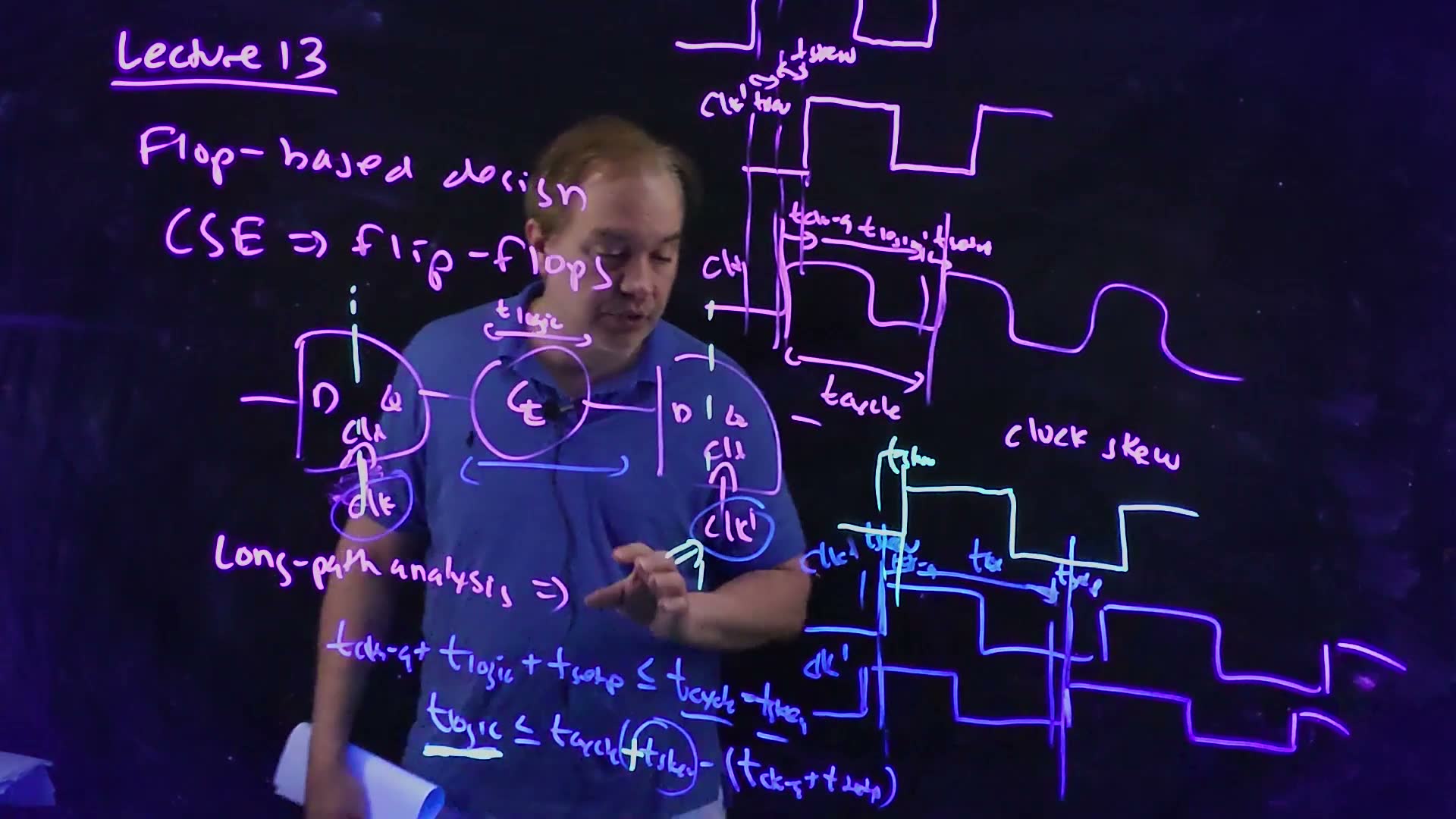
Fair copy of the board above (Lecture13 @ 08:25), mark for mark in its own layout. Black is the purple pen (the title, the flip-flop pair, the clocks at the top right and “clock skew”) and the blue pen (the circles round clk and clk′, the bracket under $C_L$CL​, the clk and clk′ rows at the lower right with their labels, and the two inequalities). Teal is the cyan pen, the later case: the second clk′ above those rows, its $t_{skew}$ after clk’s edge, the stroke that turns the circled minus into a plus, and the double arrow up into the circled clk′, which is new since 07:40. The top row runs off the top of the camera’s view and is copied as far as it shows.

The data is still launched by clk’s edge and still has to be captured by clk′‘s next edge. So the deadline is set by the capture clock, and moving that clock moves the deadline.

The long path with skew (board, 03:10–06:41)

1. Capture clock early. Suppose clk′‘s rising edges come $t_{skew}$ before clk’s (03:10–05:56) board. Launch at clk’s edge at $t = 0$0. The data leaves at $t_{clk\to Q}$ and finishes the logic at $t_{clk\to Q} + t_{logic}$tlogic​. The next capturing edge is not at $T_{cycle}$ but at $T_{cycle} - t_{skew}$tskew​, and the data must be there $t_{setup}$ before it.
2. The inequality. $t_{clk\to Q} + t_{logic} + t_{setup} \le T_{cycle} - t_{skew}$tskew​, so $t_{logic} \le T_{cycle} - t_{skew} - (t_{clk\to Q} + t_{setup})$ board. The skew comes straight off the logic’s budget.
3. Capture clock late. Now let clk′ come $t_{skew}$ after clk (06:27–06:41). The capturing edge is at $T_{cycle} + t_{skew}$tskew​, and the lecturer overwrites the circled minus: “this would actually … be a plus sign” board. The logic may take $T_{cycle} + t_{skew} - (t_{clk\to Q} + t_{setup})$tsetup​).
4. One sign for both added. Define the signed skew $\delta$ = (capture clock’s edge) − (launch clock’s edge). An early capture clock has $\delta = -t_{skew}$−tskew​, a late one $\delta = +t_{skew}$+tskew​, and both cases read $t_{clk\to Q} + t_{logic} + t_{setup} \le T_{cycle} + \delta$δ. Exam questions say “arrives 50 ps earlier” or “is delayed by 1.5 ns”; writing $\delta$ first, with its sign, stops the most common slip.

The long-path (setup) check with skew, redrawn from the board (Lecture13 @ 07:40, 08:25). Data launched at clk’s edge needs $t_{clk\to Q} + t_{logic}$ and must then be ready $t_{setup}$ before the capturing clock clk′. (a) If clk′ comes $t_{skew}$ early, the time available is $T_{cycle} - t_{skew}$tskew​. (b) If clk′ comes $t_{skew}$ late, the path gains it: $T_{cycle} + t_{skew}$tskew​. A sketch: no times are stated.

The board (Lecture13 @ 07:40)

Lecture13 @ 07:40Both cases on one board: the early clk′ gives t_cycle − t_skew; the late clk′, drawn after it, turns the circled minus into a plus.

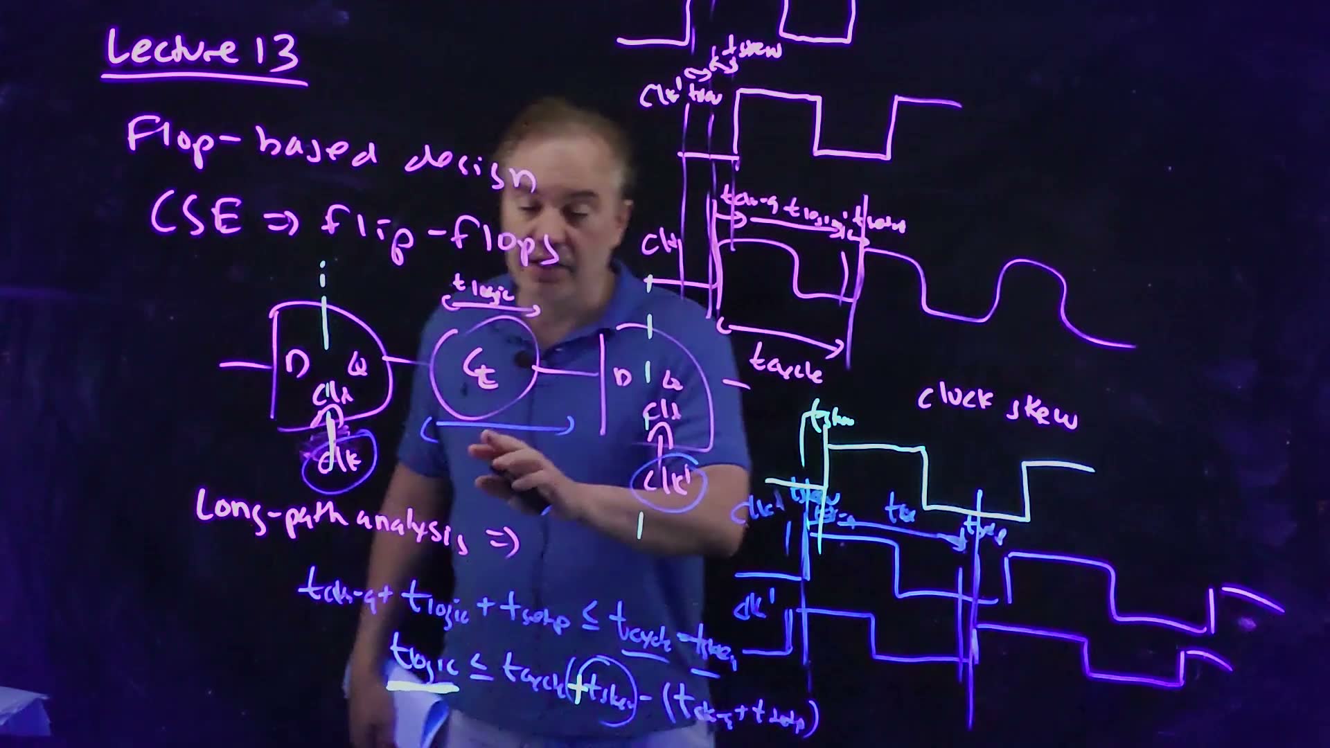
Fair copy of the board above (Lecture13 @ 07:40), mark for mark in its own layout. Black is the purple and the blue pens, as in the 08:25 copy. Teal is the cyan pen, the later case: the second clk′ above the clk and clk′ rows, its $t_{skew}$ after clk’s edge, the stroke that turns the circled minus into a plus, and the stroke below the circled clk′, which becomes a double arrow by 08:25. The top row runs off the top of the camera’s view and is copied as far as it shows.

Time is borrowed, not created

A late capture clock looks like free time. It is not (06:41). Take three flip-flops in a row, F1 on clk, F2 on clk′ (late by $t_{skew}$tskew​), F3 on clk again. Stage 1, from F1 to F2, does get $T_{cycle} + t_{skew}$tskew​. But stage 2 is launched by F2’s late edge and captured by F3’s on-time edge: it gets only $T_{cycle} - t_{skew}$tskew​. The skew moved $t_{skew}$ of time from stage 2 to stage 1, and the clock period still has to fit the worse of the two.

Skew is borrowed, not gained added (spoken at Lecture13 @ 06:41). If the middle flip-flop’s clock clk′ arrives $t_{skew}$ late, the first stage (F1 to F2) has $T_{cycle} + t_{skew}$ to work in, but the second stage (F2 to F3) launches late and must still finish by clk’s next edge: it has only $T_{cycle} - t_{skew}$tskew​. A sketch: no times are stated.

That observation has a history (07:14–08:23). If stage 1 has more logic than stage 2, a designer could skew F2’s clock on purpose to balance them. “They called it clock skew scheduling” (07:59, the lecturer’s words from the recording), and CAD companies offered it; his verdict is “terrible idea”, because every stage’s budget then depends on the clock tree’s exact delays, which vary from chip to chip. Flip-flop designs keep skew as close to zero as they can. The better way to let one stage borrow from the next is transparent latches, which Section 7 builds: there the borrowing happens by itself, without touching the clock.

A long-path failure only slows the chip

Suppose a chip comes back from fabrication and one path is too slow for the target clock. That is a late-mode failure (08:50–11:10), checked at the slow corner, and it has a simple cure: slow the clock down. $T_{cycle}$ is on the right side of the inequality, so a longer period always makes room. Manufacturers lean on this. Process variation makes some chips of the same design faster than others, so they test each chip and sell the same design at, for example, 2.8, 3.0 and 3.2 GHz (10:21) board: speed sorting. A chip that misses 3.2 GHz is not scrap; it is a 3.0 GHz part. Section 2 shows the failure that has no such cure.

The long path with skewboard

Capture clock early:

$$t_{logic} \le T_{cycle} - t_{skew} - (t_{clk\to Q} + t_{setup})$$

Capture clock late:

$$t_{logic} \le T_{cycle} + t_{skew} - (t_{clk\to Q} + t_{setup})$$

Holds when: edge-triggered flip-flops; the data is launched by one edge of the launch clock and captured by the next edge of the capture clock; checked at the slow corner (slow process, lowest V_DD, highest temperature)

The same, with signed skewadded

$$t_{clk\to Q} + t_{logic} + t_{setup} \le T_{cycle} + \delta$$

Holds when: δ = capture clock's edge − launch clock's edge (δ > 0: capture late); the same conditions

Memorize or derive. Derive it; it takes three lines, and the derivation is what stops sign slips.

1. Draw the launch edge at $t = 0$ and the capture clock’s next edge at $T_{cycle} + \delta$δ.
2. The data is ready at $t_{clk\to Q} + t_{logic}$tlogic​.
3. It must be ready $t_{setup}$ before the capture edge: $t_{clk\to Q} + t_{logic} \le T_{cycle} + \delta - t_{setup}$tsetup​.

What breaks it. A path that is meant to take more than one cycle (a multi-cycle path; not in this course), or a capture on another kind of edge. Section 3 adds a non-overlap window, and Section 4 a pulse; both change step 3.

A worked example

An added example added: $T_{cycle} = 500$ ps (2 GHz), $t_{clk\to Q} = 40$ ps, $t_{setup} = 20$ ps, and 30 ps of skew. The latch overhead is $40 + 20 = 60$ ps.

The long path with 30 ps of skew

1. Capture clock 30 ps early. $\delta = -30$ ps, so $t_{logic} \le 500 - 30 - 60 = 410$ ps. Without skew it would be 440 ps.
2. Capture clock 30 ps late. $\delta = +30$ ps, so this stage may have $t_{logic} \le 500 + 30 - 60 = 470$ ps. But the next stage is launched by this late clock and captured by an on-time one: for it, $\delta = -30$ ps and $t_{logic} \le 410$ ps.
3. A chip with a 450 ps path, in case 1. 450 ps is more than the 410 ps allowed, so the chip fails at 2 GHz. Solve the inequality for the period instead: $T_{cycle} \ge t_{logic} + t_{clk\to Q} + t_{setup} - \delta = 450 + 60 + 30 = 540$ ps. The chip works at $1/540\ \text{ps} = 1.85$ GHz and is sold as a slower part.

Traps.

• Measuring to the launch clock’s next edge. The deadline is the capture clock’s edge. With an early capture clock, using clk’s edge gives the zero-skew answer and misses the skew entirely.
• Treating a late capture clock as a gift. It hands time to this stage by taking it from the next one, whose capture clock is, relative to its launch, early.
• Thinking a long-path failure kills the chip. It only lowers the clock frequency the chip can run at.

Check yourself Two flip-flops run on a 1 GHz clock, with t_clk→Q + t_setup = 80 ps. The capture clock arrives 50 ps early. What is the largest t_logic?

$T_{cycle} = 1000$ ps and $\delta = -50$ ps, so $t_{logic} \le 1000 - 50 - 80 = 870$ ps.

Check yourself The same pair, but now the skew's sign is unknown: up to 50 ps either way, chip to chip. What t_logic is safe on every chip? And what clock period would a 900 ps path need?

The worst case for the long path is the early capture clock, $\delta = -50$ ps, so every chip works with $t_{logic} \le 870$ ps (a late clock would allow 970 ps, but some chips have the early one). For a 900 ps path: $T_{cycle} \ge 900 + 80 + 50 = 1030$ ps $= 1.03$ ns, about 971 MHz.

Check yourself Speed sorting moves a slow chip to a lower clock frequency. Why does that cure every long-path failure, and which constraint, of the two this lecture writes, is it powerless against?

The long path’s right side contains $T_{cycle}$Tcycle​, so a longer period always gives the slowest path room. The short-path (hold) constraint of Section 2 contains no $T_{cycle}$ at all, so changing the frequency does nothing for it.

2. Short paths and hold

You need

Hold time (Chapter 13 teaches it). At the capturing edge the flip-flop samples D. D must then stay stable for $t_{hold}$ after that edge, or the flip-flop may take the wrong value.

Skew and its sign (Section 1). The pair is a flip-flop on clk, logic $t_{logic}$tlogic​, and a flip-flop on clk′. In this section clk′ is late: its edge comes $t_{skew}$ after clk’s edge of the same cycle. In signed form, $\delta$ = capture clock’s edge − launch clock’s edge, here $\delta = +t_{skew}$+tskew​.

The flip-flop pair (Lecture13 @ 08:25, redrawn): launch on clk, logic $t_{logic}$tlogic​, capture on clk′. Original figure ↑

The earliest the data can move. After the launching edge, Q changes $t_{clk\to Q}$ later, and the logic passes the change on $t_{logic}$ after that. The course uses one value of each delay for both checks; it does not separate a minimum from a maximum delay.

The question. Section 1 asked whether the data arrives early enough for the next edge. This section asks the opposite: can it arrive too early, so early that the capturing flip-flop is still busy with the previous cycle’s data?

The race into the same edge

The short path (board, 11:10–15:40)

1. Look at the same cycle’s capture edge. clk’s edge at $t = 0$ launches new data. clk′‘s edge of the same cycle comes at $t_{skew}$tskew​, and it is capturing the previous cycle’s data: that data must stay on D until $t_{skew} + t_{hold}$ board.
2. The new data is racing it. The new data leaves the launching flip-flop at $t_{clk\to Q}$ and reaches D of the capturing one at $t_{clk\to Q} + t_{logic}$tlogic​. If that is before $t_{skew} + t_{hold}$thold​, the capturing flip-flop takes this cycle’s data one cycle early (13:11). The design was simulated in VHDL or Verilog on the assumption that each flip-flop advances one step per cycle; data that jumps two flip-flops in one cycle breaks that assumption, and the machine “will be completely broken”.
3. The inequality. The new data must arrive after the hold window: $t_{clk\to Q} + t_{logic} \ge t_{skew} + t_{hold}$thold​, so $t_{logic} \ge t_{skew} + t_{hold} - t_{clk\to Q}$tclk→Q​, boxed on the board (16:13) board. This is a minimum delay: the logic must be at least this slow.
4. Without skew it is rarely a problem (said at 30:55). With $t_{skew} = 0$ the bound is $t_{hold} - t_{clk\to Q}$tclk→Q​, and a normal flip-flop has $t_{clk\to Q} > t_{hold}$thold​, so the bound is negative: any logic, even none, is slow enough. Skew is what turns the minimum positive.

The short-path (hold) check when the capture clock clk′ is late by $t_{skew}$tskew​, redrawn from the board (Lecture13 @ 18:13). Data launched at clk’s edge can reach the capturing flip-flop as early as $t_{clk\to Q} + t_{logic}$ later. It must not arrive before clk′‘s own edge plus $t_{hold}$ (the dotted line), or it overwrites the value being captured: $t_{clk\to Q} + t_{logic} \ge t_{skew} + t_{hold}$thold​. A sketch: no times are stated.

The board (Lecture13 @ 18:13)

Lecture13 @ 18:13The short path with a late capture clock, the boxed minimum logic delay, and the notes on shift registers, padding and the early-mode corner.

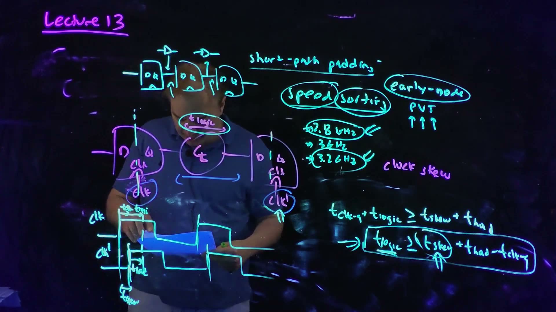
Fair copy of the board above (Lecture13 @ 18:13), mark for mark in its own layout. Teal is the cyan pen, everything new on this board: the shift register with a buffer drawn over each link, the notes (short-path padding, speed sorting, 2.8, 3 and 3.2 GHz, early-mode PVT), the circle round $t_{logic}$tlogic​, the double arrow under clk′, the clk and clk′ rows with $t_{c\text{-}q}$tc-q​, $t_{logic}$tlogic​, $t_{hold}$ and $t_{skew}$tskew​, and the two inequalities. Black is what is left of the long-path board: the purple pen (the title, the flip-flop pair, “clock skew” and a few remnants at the left) and the blue pen (the circles round clk and clk′ and the bracket under $C_L$CL​). The clock rows, partly behind the sheet the lecturer holds at 18:13, are read from 18:42.

Shift registers and short-path padding

The worst case is no logic at all (15:40) board: a shift register, flip-flops chained Q to D, has $t_{logic} = 0$0. With a late capture clock it fails as soon as $t_{clk\to Q} < t_{skew} + t_{hold}$thold​. The fix is to slow the short paths down on purpose: put buffers in each Q-to-D wire until the minimum is met. The board calls this short-path padding (16:53).

(a) A shift register: flip-flops wired Q to D with no logic, $t_{logic} = 0$0, the worst case for the hold check, since any late skew larger than $t_{clk\to Q} - t_{hold}$ breaks it. (b) Short-path padding: a buffer in each connection adds delay to the short path, so the data cannot race through on a late clock edge. Redrawn from the board’s notes (Lecture13 @ 18:13; the frame is folded under the short-path figure of this section).

Checked at the fast corner

A long path fails when the delays are largest, so it is checked at the slow corner. A short path fails when the delays are smallest, so it is checked at the fast corner (17:44): the board writes “early-mode” and “PVT ↑↑↑”, and the lecturer names the corner in words: “the fastest corner, the fast [process], the highest voltage and the lowest temperature”.

Check	Fails when the delays are	Corner (process, $V_{DD}$VDD​, temperature)
Long path, late mode (Section 1)	largest	slow, lowest, highest
Short path, early mode (this section)	smallest	fast, highest, lowest

A chip killer

Now ask what a short-path failure on a finished chip can be cured with (17:23): “Can I slow the clock down? No. Can I speed the clock up? … No. … I’m stuck.” Look at the inequality: $t_{logic} \ge t_{skew} + t_{hold} - t_{clk\to Q}$tclk→Q​. There is no $T_{cycle}$ in it. The race happens between two edges of the same cycle, so no period makes it go away. Short-path problems “are chip killers” (18:02): the chip is scrap, unless the designers built in a knob to change the clock edges themselves, which is the subject of Section 3.

In signed form added, the short path is $t_{clk\to Q} + t_{logic} \ge t_{hold} + \delta$δ. A late capture clock ($\delta > 0$δ>0) makes it harder. An early capture clock ($\delta < 0$δ<0) makes it easier: the capture edge has come and gone before the new data could arrive. The same early clock costs the long path, as Section 1 showed. Skew always helps one check and hurts the other.

The short path with skewboard

$$t_{logic} \ge t_{skew} + t_{hold} - t_{clk\to Q}$$

Holds when: edge-triggered flip-flops; the capture clock late by t_skew; checked at the fast corner (fast process, highest V_DD, lowest temperature); no T_cycle appears, so no clock frequency fixes a failure

The same, with signed skewadded

$$t_{clk\to Q} + t_{logic} \ge t_{hold} + \delta$$

Holds when: δ = capture clock's edge − launch clock's edge; an early capture clock (δ < 0) helps hold

Memorize or derive. Memorize the rule of thumb (spoken, 30:55): without skew, a flip-flop with $t_{clk\to Q} \ge t_{hold}$ has no hold problem. Derive the inequality:

1. The new data reaches D at $t_{clk\to Q} + t_{logic}$ after the launch edge.
2. The capture edge of the same cycle is at $\delta$δ, and the old data must stay until $\delta + t_{hold}$thold​.
3. So $t_{clk\to Q} + t_{logic} \ge \delta + t_{hold}$thold​.

A worked example

The flip-flops of Section 1’s example added: $t_{clk\to Q} = 40$ ps, now with $t_{hold} = 15$ ps.

Hold with a late capture clock

1. No skew. $t_{logic} \ge 0 + 15 - 40 = -25$ ps. A negative minimum is no constraint: even a direct Q-to-D wire is safe.
2. Capture clock 30 ps late. $t_{logic} \ge 30 + 15 - 40 = 5$ ps. A shift register ($t_{logic} = 0$tlogic​=0) fails by 5 ps: its new data arrives at 40 ps, while the old data must stay until 45 ps. Pad each Q-to-D wire with at least 5 ps of buffer delay.
3. 60 ps late. $t_{logic} \ge 60 + 15 - 40 = 35$ ps: now every path between these flip-flops, not only the shift register, needs at least 35 ps.
4. Slow the clock to 1 GHz? None of the three numbers changes, because none contains $T_{cycle}$Tcycle​. The 2 GHz chip and the 1 GHz chip fail alike.

Traps.

• Checking hold against the next cycle’s edge. That is the setup check of Section 1. Hold is against the capture edge of the same cycle.
• Putting $T_{cycle}$ into the hold check. It does not belong there, which is why the failure cannot be clocked away.
• Checking hold at the slow corner. The slow corner makes the data late, which is safe for hold. The dangerous chip is the fast one.
• Thinking a late capture clock is harmless because it helps the long path. It hurts the short path by exactly the amount it helps the long one.

Check yourself A flip-flop has t_clk→Q = 60 ps and t_hold = 20 ps. How much skew can a shift register built from it tolerate, and in which direction?

With $t_{logic} = 0$0, the constraint is $60 \ge t_{skew} + 20$20, so the capture clock may be up to 40 ps late. An early capture clock never hurts hold.

Check yourself The same flip-flops, in a shift register whose clock has 100 ps of jitter, treated as skew in the worst direction. Is padding needed, and how much? Then: would halving the clock frequency help?

The worst direction for hold is a late capture clock, $\delta = +100$ ps. The minimum logic delay is $100 + 20 - 60 = 60$ ps, and a shift register has none, so each Q-to-D wire needs at least 60 ps of padding. Halving the frequency changes nothing: $T_{cycle}$ does not appear in the hold check.

Check yourself Why is the fast corner the right one for the short path?

The short path fails when the new data arrives too soon. The data arrives soonest when $t_{clk\to Q}$ and $t_{logic}$ are smallest, and that is the fast process, the highest $V_{DD}$ and the lowest temperature.

3. Two-phase clocks and the non-overlap window

You need

The master–slave flip-flop (Chapter 13 teaches it). A flip-flop is two transparent-high latches in a row: the master on one clock phase, the slave on the other. A transparent-high latch passes D to Q while its clock is high and holds when its clock falls. The flip-flop captures when the master closes and launches when the slave opens; with complementary phases both happen at the same instant, which is the flip-flop’s edge.

The short path of Section 2. Data launched at one edge must not reach the next flip-flop before that flip-flop’s capture edge of the same cycle plus $t_{hold}$thold​. With the capture clock late by $t_{skew}$tskew​: $t_{clk\to Q} + t_{logic} \ge t_{skew} + t_{hold}$thold​. No $T_{cycle}$ appears, so a failure cannot be fixed by the clock frequency.

The short path with the capture clock late (Lecture13 @ 18:13, redrawn): the new data must clear $t_{skew} + t_{hold}$thold​. Original figure ↑

The long path and its overhead (Chapter 13 derives it; Section 1 here adds skew). Without skew, $t_{logic} \le T_{cycle} - (t_{clk\to Q} + t_{setup})$tsetup​).

The question. Section 2 ended with a chip that has a hold failure and no cure. Can a design keep a knob that repairs a short-path failure after the chip is made? It can, if the flip-flops’ two latch clocks are made locally, so that their edges can be moved apart.

A flip-flop as two latches on two phases

Moving one edge (board, 18:00–25:24)

1. Split each flip-flop (18:42) board. Draw the pair as four latches: φ1 (master) and φ2 (slave), the logic, then φ1′ and φ2′. φ1 and φ2 are generated locally from the one global clock wire, nominally “180 degrees out of phase” (19:47): complementary. φ1′ and φ2′ are the same clocks at the receiving pair, late by $t_{skew}$tskew​.
2. Find the two edges that race (21:09) board. The launch is φ2’s rising edge: the slave opens and lets the new data out. The hold-critical capture is φ1′‘s falling edge: the receiving master closes on the previous cycle’s data. φ1′ is late, so its falling edge comes $t_{skew}$ after the launch, and with little logic the new data slips into the receiving master in the same cycle. That is Section 2’s failure, seen at latch level.
3. Pull φ1’s falling edge earlier (22:40–24:39) board. Shorten φ1’s high time, so φ1 falls before φ2 rises. Now there is a window in which both phases are low: the non-overlap window. The board calls its length $t_{overlap}$toverlap​, although it measures the time with no overlap. φ2’s rising edge does not move, so the launch stays where it was. The receiving pair’s φ1′ is made the same way, so its falling edge, the hold-critical capture, moves $t_{overlap}$ earlier too.
4. Hold is repaired added. The capture edge now comes $t_{overlap}$ sooner after the launch, so the race has $t_{overlap}$ more margin: $t_{overlap} + t_{clk\to Q} + t_{logic} \ge t_{skew} + t_{hold}$thold​. Make the window wide enough and any hold failure goes away. The board shows the window “big enough”; this inequality is Section 2’s, measured from the moved edge.

A flip-flop pair built from two-phase latches, with the capturing pair’s clocks φ1′, φ2′ late by the skew, redrawn from the board (Lecture13 @ 24:39, 25:24). (a) Data launches when φ2 opens the first slave and can race into the next master, which stays open until φ1′ falls, $t_{skew}$ later: a hold hazard. (b) Moving φ1’s falling edge earlier (and φ1′‘s with it) opens a non-overlap window, the dead time $t_{overlap}$toverlap​, in which both phases are low; now the next master closes before the launch. A sketch: no times are stated.

The board (Lecture13 @ 25:24)

Lecture13 @ 25:24The moved φ1 edge (orange on the board), the non-overlap window t_overlap, and the dead time it costs the long path.

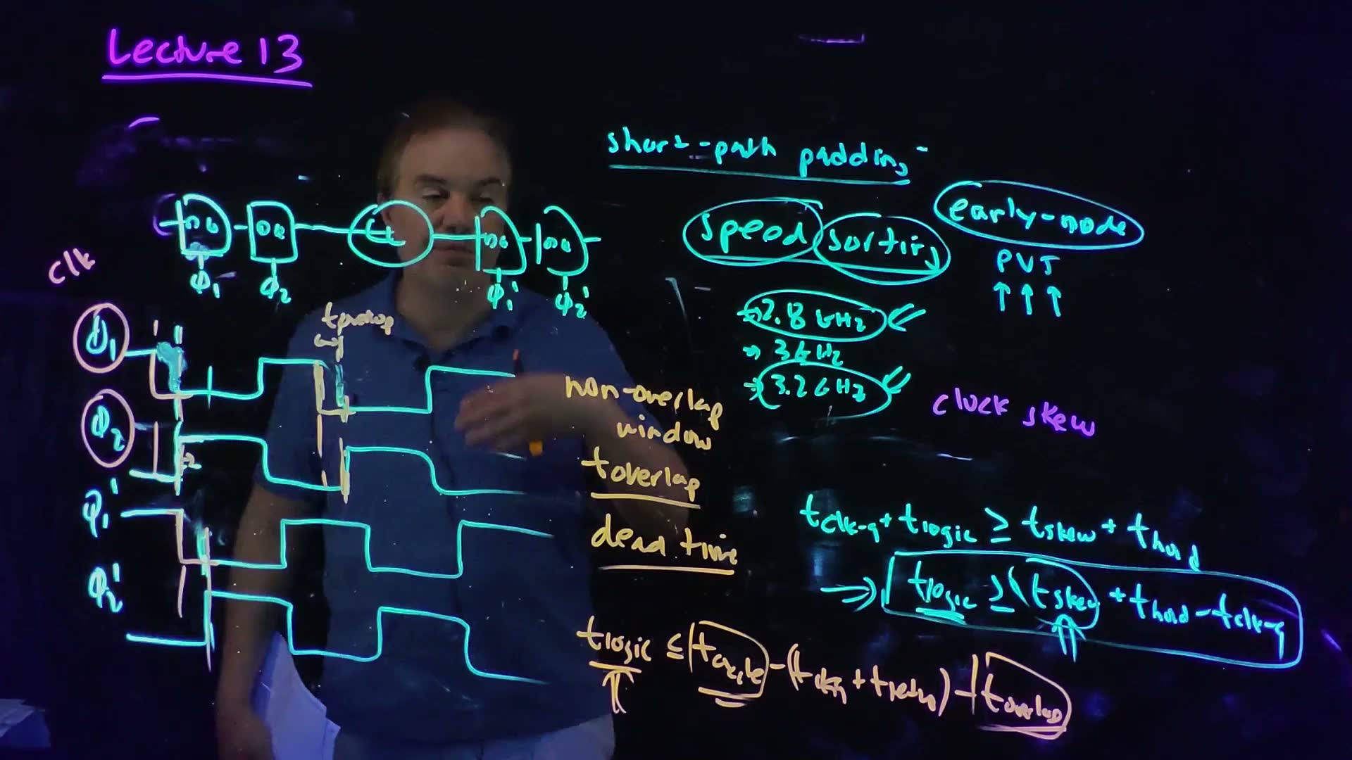
Fair copy of the board above (Lecture13 @ 25:24), mark for mark in its own layout. Black is the cyan pen (the latch row, the four clock rows and their labels, and the short-path notes and inequalities left from 18:13) and the purple pen (the title, “clock skew”, “clk” and the circles round φ1 and φ2). Orange is the orange pen, the two-phase working: the falling edges of φ1 and φ1′ drawn earlier, with their guides and the low stretches they add, $t_{overlap}$ over φ1’s second falling edge, “non-overlap window”, $t_{overlap}$ and “dead time”, and the long-path inequality with its circles and marks. The cyan edges the orange ones replace are still on the board, beside them; where φ1’s first edge was rubbed out only a smudge is left, which is not copied.

The price: dead time

Nothing is free (23:40–25:24) board. During the window the master is already closed and the slave not yet open, so no data moves anywhere: the board labels it dead time. The long path pays for it. Its deadline is the next closing edge of φ1′, which also moved $t_{overlap}$ earlier, while the launch did not. So, written as the board writes it, without skew:

$$t_{logic} \le T_{cycle} - (t_{clk\to Q} + t_{setup}) - t_{overlap}.$$

So the repaired chip works, but at a lower clock frequency: the period must grow by the width of the window. Designers accept that, because the alternative is scrap. The lecturer says “most modern microprocessors will have such a capability”: a way to widen the window after fabrication.

The long path with a non-overlap windowboard

$$t_{logic} \le T_{cycle} - (t_{clk\to Q} + t_{setup}) - t_{overlap}$$

Holds when: master–slave flip-flops on locally generated φ1, φ2; the window between φ1's falling edge and φ2's rising edge has length t_overlap; written without skew (add δ as in Section 1)

The same, with signed skewadded

$$t_{clk\to Q} + t_{logic} + t_{setup} \le T_{cycle} + \delta - t_{overlap}$$

Holds when: δ = capture pair's edge − launch pair's edge, as in Section 1; the window moves every capturing edge t_overlap earlier relative to its launch

The window a hold failure needsadded

$$t_{overlap} \ge t_{skew} + t_{hold} - t_{clk\to Q} - t_{logic}$$

Holds when: the receiving pair's clocks late by t_skew; the window delays the launch relative to the hold-critical capture edge; t_logic is the shortest path between the pairs; checked at the fast corner

Memorize or derive. Derive all three from one picture: the window moves the capturing edge $t_{overlap}$ earlier relative to the launch, and the skew moves it by $\delta$δ. For hold, that is $t_{overlap}$ of extra margin; for setup, $t_{overlap}$ of lost time.

How a local generator makes the window

The lecture says the clocks are generated locally “from my single-wire global clock” (24:58) but draws no circuit. Past finals do (FN12-7), so here is the usual one added. It needs only the NOR’s truth table: a NOR’s output is high only when both inputs are low.

Two NOR gates are cross-coupled through delay blocks. $\phi_1 = \text{NOR}(\phi, \Delta_1(\phi_2))$ and $\phi_2 = \text{NOR}(\overline{\phi}, \Delta_2(\phi_1))$NOR(ϕ​,Δ2​(ϕ1​)), where $\Delta_1(\phi_2)$ means φ2 delayed by $\Delta_1$Δ1​.

The generator, edge by edge (added; gate delays ignored)

1. φ rises. φ is an input of φ1’s NOR, so φ1 falls at once. φ2’s NOR sees $\overline\phi$ low, but its other input is φ1 delayed by $\Delta_2$Δ2​, which is still high. φ2 rises only $\Delta_2$ after φ1 fell.
2. φ falls. Now $\overline\phi$ is high, so φ2 falls at once. φ1’s NOR sees φ low, but its other input, φ2 delayed by $\Delta_1$Δ1​, is still high: φ1 rises $\Delta_1$ after φ2 fell.
3. Why the phases never overlap. Each phase can rise only after it has seen the other one low, through its delay block. So there are two windows each cycle: $\Delta_2$ after φ1 falls, and $\Delta_1$ after φ2 falls.
4. How it makes the window. The generator delays the slave’s opening: φ1 falls with φ, and φ2 rises $\Delta_2$ later. The board did the opposite, moving φ1’s falling edge earlier and leaving φ2’s rise in place. Only the gap between the master’s closing and the slave’s opening matters, for hold and for the dead time alike, so the two are the same fix: in the generator the launch moves later, on the board the capture edge moves earlier.
5. Which window cures hold. It is the gap from the master’s closing edge to the slave’s opening edge. In this generator φ2 is high while φ is high, so if the master is on φ1 (the board’s flip-flop), that gap is $\Delta_2$Δ2​; if a circuit puts the master on φ2, it is $\Delta_1$Δ1​. Read the figure before choosing.

A non-overlapping two-phase clock generator added (the topology of FN12-7’s figure). Each NOR is held low by its own input clock and by the other phase delayed, so φ1 rises only $\Delta_1$ after φ2 has fallen, and φ2 only $\Delta_2$ after φ1 has fallen: two windows each cycle in which both phases are low. The timing is drawn with $\Delta_1 = 0.10\,T$ and $\Delta_2 = 0.06\,T$0.06T, ignoring the gates’ own delays.

A worked example

An added example added: master on φ1, slave on φ2; $t_{clk\to Q} = 40$ ps, $t_{hold} = 15$ ps, $t_{setup} = 20$ ps; the receiving pair’s clocks are 80 ps late; the shortest logic between the pairs is 20 ps; $T_{cycle} = 500$ ps.

Sizing the window and paying for it

1. Check hold without a window. The new data arrives $40 + 20 = 60$ ps after the launch. The old data must stay until $80 + 15 = 95$ ps. $60 < 95$95: it fails, by 35 ps.
2. The window it needs. $t_{overlap} \ge 80 + 15 - 40 - 20 = 35$ ps.
3. The long path into the late pair. The board writes the long path without skew, which would give $500 - 60 - 35 = 405$ ps. But this stage’s capture clock is late, $\delta = +80$ ps, so with the signed form it gets $t_{logic} \le 500 + 80 - 60 - 35 = 485$ ps.
4. The stage after it pays. The next stage launches from the late pair and captures at an on-time pair: $\delta = -80$ ps. With the same window (every generator is built alike), it gets $t_{logic} \le 500 - 80 - 60 - 35 = 325$ ps; without the window it would have 360 ps. The window costs every stage 35 ps; the skew moves 80 ps from the second stage to the first, as in Section 1.
5. If a 440 ps path sits in that second stage. It fits only if $T_{cycle} \ge 440 + 60 + 35 + 80 = 615$ ps: the repaired chip runs at 1.63 GHz instead of 2 GHz. A working chip at a lower bin, instead of scrap.

Traps.

• Moving φ2’s falling edge. That opens the other window, between the slave’s closing and the master’s opening, and does not delay this launch relative to this capture.
• Forgetting the receiving clocks. φ1′ is generated the same way, so its edge moves too; it is that edge, the capture, that moves away from the launch.
• Treating the window as free. Every picosecond of window is a picosecond of dead time in every cycle.
• Reading $t_{overlap}$ as an overlap. The board’s name measures the time when no phase is high.

Check yourself In the two-phase flip-flop pair with φ1's falling edge moved earlier, which edge launches the short path, and which edge must it not beat?

The launch is φ2’s rising edge at the first pair (its slave opens). The edge it must not beat, plus $t_{hold}$thold​, is φ1′‘s falling edge at the receiving pair (its master closes on the old data). The window moves that falling edge earlier, away from the launch.

Check yourself A flip-flop has t_clk→Q = 30 ps, t_hold = 10 ps and t_setup = 15 ps. The receiving pair's clocks are 70 ps late, and the shortest path between the pairs has no logic. How wide must the window be? Then, at T_cycle = 400 ps, what is the longest logic into the late pair, and in the stage after it?

Hold: $t_{overlap} \ge 70 + 10 - 30 - 0 = 50$ ps. Into the late pair, $\delta = +70$ ps: $t_{logic} \le 400 + 70 - (30 + 15) - 50 = 375$ ps. The stage after it captures on time, $\delta = -70$ ps: $t_{logic} \le 400 - 70 - 45 - 50 = 235$ ps. (The board’s formula, without skew, gives 305 ps for both; neither stage actually has it.)

Check yourself In the cross-coupled NOR generator, φ falls. Which phase moves first, and how long until the other one rises?

$\overline\phi$ rises, so φ2’s NOR output falls at once. φ1 rises only when φ2, delayed by $\Delta_1$Δ1​, has gone low: $\Delta_1$ after φ2 fell.

4. Pulsed latches

You need

The transparent latch (Chapter 13 teaches it). While its clock is high, Q follows D; when the clock falls, the latch holds. Its setup and hold times are measured around the closing (falling) edge, and $t_{clk\to Q}$ from the opening (rising) edge.

Why a flip-flop costs two latches. A master–slave flip-flop passes the data through both latches, so its overhead $t_{clk\to Q} + t_{setup}$ is that of a two-latch structure.

The short path with skew (Section 2). With the capture clock late by $t_{skew}$tskew​, the new data must not arrive before the capture edge plus $t_{hold}$thold​: $t_{logic} \ge t_{skew} + t_{hold} - t_{clk\to Q}$tclk→Q​. Without skew, a flip-flop has $t_{clk\to Q} > t_{hold}$thold​, so the bound is negative.

The short path with the capture clock late (Lecture13 @ 18:13, redrawn): the new data must clear $t_{skew} + t_{hold}$thold​. Original figure ↑

The question. A flip-flop is two latches. Could one latch do the job, if its clock is high only for a moment? It can, and it is faster; but the moment it is open is also a moment in which a fast path can race through.

One latch on a short pulse

Pulse-mode clocking (board, 25:40–28:00)

1. One latch, one short clock (26:41) board. Take a single D latch and clock it with lclk, a local clock that is high for only a short pulse, once per cycle. The circuit that makes the pulse has several names: a one-shot, a clock chopper, a clock shaper (27:19). The concept board draws one pulse at each rising edge of clk. While the latch is open for so short a time, it behaves like an edge-triggered flip-flop.
2. The gain (spoken). The data crosses one latch instead of two, so $t_{clk\to Q}$ and the overhead are one latch’s. Every cycle gets that time back for logic.

Pulse-mode clocking, redrawn from the board (Lecture13 @ 27:39). A single latch is clocked by lclk, a short pulse made once per cycle by a one-shot, so the latch is transparent only briefly and acts almost like an edge-triggered flip-flop. This concept board puts the pulse at each rising edge of clk; the NOR chopper of Section 5 makes it after each falling edge instead.

The board (Lecture13 @ 27:39)

Lecture13 @ 27:39Pulse-mode clocking: one latch on lclk, with a short pulse at each rising edge of clk (right).

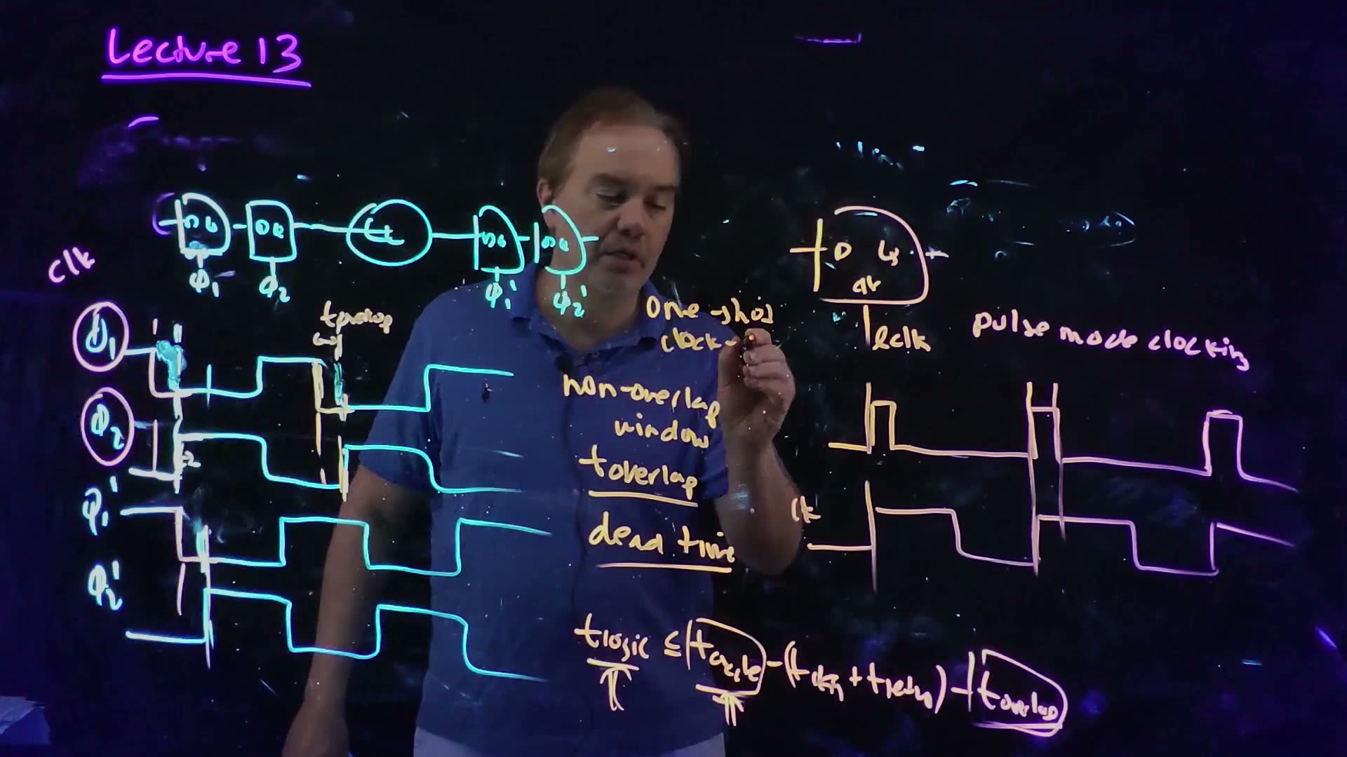
Fair copy of the board above (Lecture13 @ 27:39), mark for mark in its own layout. The left half is the 25:24 board, with the double arrow under $t_{cycle}$ finished at 25:39; the short-path notes at the right have been erased for the pulse-mode board. Black is the cyan pen (the latch row and the four clock rows with their labels) and the purple pen (the title, “clk” and the circles round φ1 and φ2). Orange is the orange pen: the two-phase working, and at the right the latch on lclk, lclk with a short pulse at each rising edge of clk, clk, “pulse mode clocking” and “One-shot clock-”. That pen looks pale yellow near the middle of the board and turns lavender towards the right edge of the view; it is one pen. “clock-” is being written at 27:39 and is copied as it stands; by 28:49 it reads “clock-chopper”.

How the pulse is made, and on which edge, is Section 5: the chopper the lecturer draws there, repeated here, puts its pulse after clk’s falling edge, although this concept board draws it at the rising edge.

The clock chopper (Lecture13 @ 34:41, redrawn): a NOR of clk and clk delayed through three inverters. Section 5 explains it. Original figure ↑

The pulse widens the race

The short path of a pulsed latch (board, 28:00–32:10)

1. Two pulsed latches with skew (28:52) board. The launching latch is on lclk; the receiving latch is on lclk′, late by $t_{skew}$tskew​, and its pulse is $t_{pulse}$ wide.

2. Where the old data must stay. The receiving latch is transparent for the whole pulse, so it is still taking in the old data until its pulse closes, at $t_{skew} + t_{pulse}$ after the launch, and then for $t_{hold}$ more. The new data, which leaves the launching latch at $t_{clk\to Q}$ after its pulse opens, must not arrive before then.

3. The inequality (30:00) board. $t_{clk\to Q} + t_{logic} \ge t_{skew} + t_{pulse} + t_{hold}$thold​, so

   $$t_{logic} \ge t_{skew} + t_{pulse} + t_{hold} - t_{clk\to Q},$$

   with $t_{pulse}$ circled on the board. Even with no skew, the pulse width is added to the minimum delay.

4. Two-sided (30:27) board. The logic now has a maximum (the long path) and a minimum that is no longer negligible: “a two-sided timing constraint”. A flip-flop without skew rarely has a minimum (Section 2); skew gives it one; a pulse makes it larger still.

5. And the long path borrows added. The receiving latch accepts data until its pulse closes, so a stage whose data arrives late, inside the pulse, is still captured: its deadline is $t_{setup}$ before the pulse closes. But that data leaves the receiving latch as late as it arrived, so the next stage starts late by the same amount. The pulse lends time to one stage by taking it from the next, as skew did in Section 1 and as transparent latches do in Section 7; along a pipeline it creates no time. The lecture names only the lower overhead.

The hold check with pulsed latches, redrawn from the board (Lecture13 @ 30:54). The capturing latch stays transparent for the whole pulse, so data launched at lclk’s rising edge must not arrive before lclk′‘s pulse has ended and $t_{hold}$ has passed (the dotted line): $t_{clk\to Q} + t_{logic} \ge t_{skew} + t_{pulse} + t_{hold}$thold​. A sketch: no times are stated.

The board (Lecture13 @ 30:54)

Lecture13 @ 30:54The pulsed short path: the pulse width joins the hold requirement, and the timing becomes two-sided.

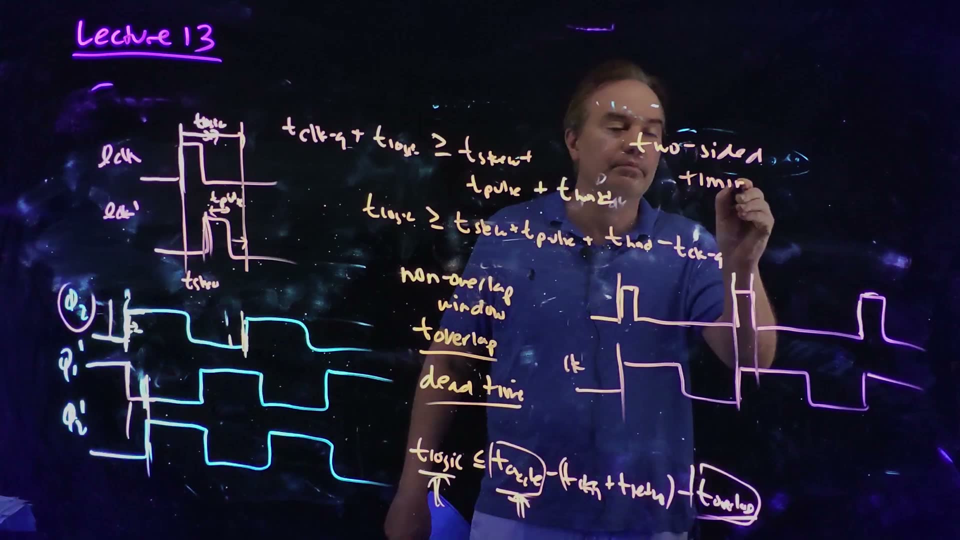
Fair copy of the board above (Lecture13 @ 30:54), mark for mark in its own layout. Since 27:39 the latch row, the φ1 row and the pulse-mode latch with its notes have been erased; the rest of the lower half, and lclk and clk at the right, are kept. Black is the cyan pen (the φ2, φ1′ and φ2′ rows and their labels) and the purple pen (the title and the circle round φ2). Orange is the orange pen: the two-phase working and the long-path inequality kept from before, and the new pulsed short path at the top: lclk and the later lclk′ with $t_{logic}$tlogic​, $t_{pulse}$ and $t_{skew}$tskew​, the two inequalities, and “two-sided timin”. That pen reads pink to lavender towards the left and right of the view and orange in the middle; it is one pen. “timin” is being written at 30:54 and is copied as it stands; by 31:39 the note reads “two-sided timing constraint”, and by 32:07 $t_{pulse}$ in the second inequality is circled.

The short path of a pulsed latchboard

$$t_{logic} \ge t_{skew} + t_{pulse} + t_{hold} - t_{clk\to Q}$$

Holds when: pulsed latches, transparent for t_pulse; the receiving pulse late by t_skew; t_clk→Q measured from the launching pulse's opening; checked at the fast corner

The same, with signed skewadded

$$t_{clk\to Q} + t_{logic} \ge \delta + t_{pulse} + t_{hold}$$

Holds when: δ = receiving pulse's opening − launching pulse's opening (δ < 0: the receiving pulse is early, which allows a wider pulse)

The long path of one pulsed stageadded

$$t_{clk\to Q} + t_{logic} + t_{setup} \le T_{cycle} + \delta + t_{pulse}$$

Holds when: data captured if it reaches the receiving latch t_setup before its pulse closes; whatever arrives after the pulse opens is borrowed from the next stage, which starts that much late; δ as above

Memorize or derive. Derive the long path from Section 1’s: the capture deadline is now the end of the pulse, and any use of the pulse is a loan from the next stage. Derive the short path from Section 2’s picture in one move: the capture edge is now the end of the pulse, so add $t_{pulse}$ to the right side. Turned round, it gives the widest pulse a design allows: $t_{pulse} \le t_{clk\to Q} + t_{logic,min} - t_{hold} - \delta$δ.

A worked example

An added example added: $t_{pulse} = 60$ ps, $t_{hold} = 15$ ps, $t_{clk\to Q} = 30$ ps.

The pulse as a hold cost

1. No skew. $t_{logic} \ge 0 + 60 + 15 - 30 = 45$ ps. Every path, even with perfect clocks, needs 45 ps of logic. Compare Section 2’s flip-flop, whose minimum was $-25$ ps: no constraint at all.
2. The receiving pulse 30 ps late. $t_{logic} \ge 30 + 60 + 15 - 30 = 75$ ps.
3. Turned round: the widest pulse. Suppose instead the shortest logic between two pulsed latches is 50 ps and the receiving pulse is 20 ps early ($\delta = -20$δ= ps). From $t_{clk\to Q} + t_{logic} \ge \delta + t_{pulse} + t_{hold}$thold​: $t_{pulse} \le 30 + 50 + 20 - 15 = 85$ ps. The early receiving clock allows a pulse 20 ps wider than perfect clocks would.

Traps.

• Measuring hold from the pulse’s rising edge. The receiving latch keeps listening until its pulse closes: hold is measured from the falling edge.
• The sign of an early receiving clock. It moves the closing edge earlier, so it allows a wider pulse, not a narrower one.
• Thinking pulsed latches remove the hold problem. They remove one latch’s overhead and make the hold problem worse.

Check yourself A wider pulse lets a slow stage's data arrive later and still be captured. Why is that not free time, and what does the wider pulse cost the short path?

Data that arrives inside the receiving pulse is captured, but it leaves that latch as late as it arrived, so the next stage starts late by the same amount: the time is borrowed from the next stage, as with skew in Section 1. Meanwhile early data from the next cycle can also get in while the pulse is open, so the short path’s minimum rises by $t_{pulse}$tpulse​.

Check yourself Pulsed latches with t_clk→Q = 25 ps and t_hold = 10 ps; the shortest logic is 40 ps; skew is up to 15 ps either way. What is the widest pulse that works on every chip? If the chopper's inverters are 20 ps each, how many may its chain have?

The worst case for hold is the receiving pulse 15 ps late: $t_{pulse} \le 25 + 40 - 10 - 15 = 40$ ps. A chopper’s chain must have an odd number of inverters (Section 5): one gives 20 ps, three give 60 ps, which is too wide. So one inverter, a 20 ps pulse.

Check yourself Which of the constraints in this section contains T_cycle?

Only the long path (step 5). The pulsed short path, like the flip-flop’s, has no $T_{cycle}$Tcycle​: a pulse that is too wide is a chip killer unless its width can be changed.

Try it: one pair, both checks

This interactive pair added puts Sections 1 to 4 on one time axis: a launching element on clk and a capturing one on clk′, with signed skew $\delta$δ. Its defaults are this chapter’s flip-flops ($t_{clk\to Q} = 40$tclk→Q​= ps, $t_{setup} = 20$ ps, $t_{hold} = 15$ ps, $T_{cycle} = 500$ ps) with the capture clock 30 ps late. Drag $\delta$ through zero and watch the two checks trade: the long-path limit moves up as the short-path wall moves out. Widen the non-overlap window to cure a hold failure and see what the long path pays. Switch to pulsed latches and widen the pulse: both bands move to the end of the capture pulse. The slow-corner and fast-corner checks are drawn on one picture with one set of delays, as the course does.

flip-flops (§1–§3)pulsed latches (§4)

skew δ, capture − launch (+ late)

30 ps

t_logic

200 ps

T_cycle

500 ps

t_clk→Q

40 ps

t_setup

20 ps

t_hold

15 ps

non-overlap window t_overlap

0 ps

Long path (slow corner): the data is ready at 240 ps and must be ready by 510 ps, so t_logic ≤ 470 ps. Met, with 270 ps to spare.

Short path (fast corner): the new data must not arrive before 45 ps, so t_logic ≥ 5 ps. Met, with 195 ps to spare.

The data leaves the launching element t_clk→Q after its edge (grey bar) and passes the logic (coloured bar). Orange band: the capturing element is still taking the previous cycle's data (its closing edge plus t_hold); blue band: the setup window before the next capturing edge. The capturing flip-flop's phases are drawn below clk′: its master φ1′ closes t_overlap before its slave φ2′ opens (grey: the non-overlap window, dead time). Hold is checked against the master's close and gains t_overlap; the long path loses it. Added: the board writes each case separately; here δ, t_overlap and t_pulse combine.

5. The clock chopper

You need

The NOR gate. A NOR’s output is high only when both inputs are low; if either input is high, the output is low.

Inverter delay (Chapter 7 teaches it). Each inverter delays the edge passing through it by its delay, here $t_{inv}$tinv​, and inverts it. A chain of an odd number of inverters inverts its input and delays it by the sum of their delays.

Why a pulse is wanted (Section 4). A pulsed latch is a single latch that is open only for a short pulse on its local clock lclk, once per cycle. The pulse’s width $t_{pulse}$ enters the hold constraint, $t_{logic} \ge t_{skew} + t_{pulse} + t_{hold} - t_{clk\to Q}$tclk→Q​, so the width must be controlled.

Pulse-mode clocking (Lecture13 @ 27:39, redrawn): one latch on lclk, a short pulse once per cycle. The concept board draws the pulse at the rising edge; this section finds where the board’s circuit really puts it. Original figure ↑

The question. How does a circuit turn a 50%-duty clock into one short pulse per cycle, and what sets the pulse’s width?

Two inputs that are both low for a moment

The clock chopper (one-shot), redrawn from the board (Lecture13 @ 34:41). clk feeds a NOR directly and through three inverters, so the NOR’s second input is $\overline{\mathrm{clk}}$ delayed by $3t_{inv}$3tinv​. A NOR goes high only when both inputs are low, and that happens for $3t_{inv}$ after each falling edge of clk: lclk is a short pulse there, and there is none at the rising edge, where $\overline{\mathrm{clk}}$ is still high. The timing is drawn with a chain delay of 0.1 of the period.

The board (Lecture13 @ 34:41)

Lecture13 @ 34:41The clock chopper and its waveforms: lclk pulses after each falling edge of clk (right). The φ clocks and the dead-time inequality at the lower left are left from Section 3.

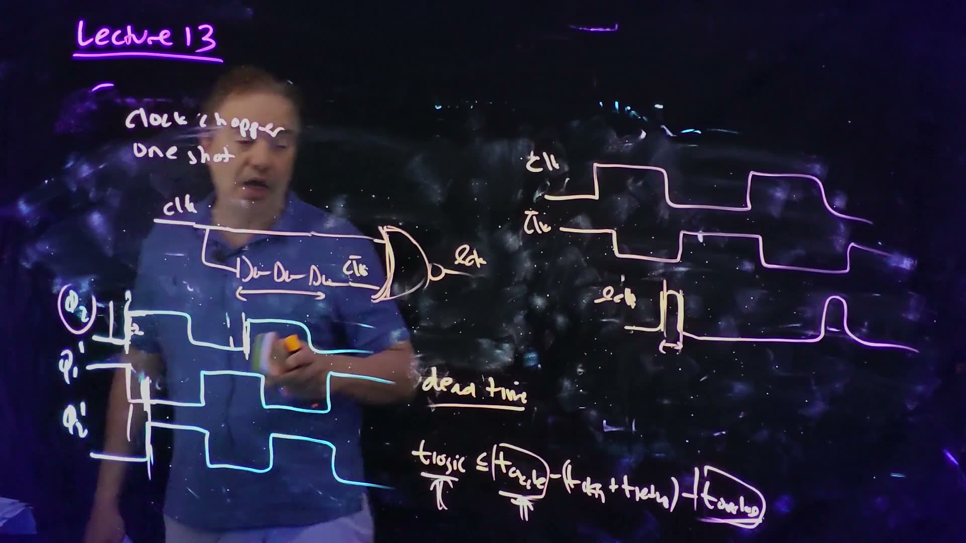
Fair copy of the board above (Lecture13 @ 34:41), mark for mark in its own layout. Since 30:54 the pulsed short path, “two-sided timing constraint”, “non-overlap window”, $t_{overlap}$ and lclk and clk at the right have been erased; the three φ rows, “dead time” and the long-path inequality are kept. Black is the cyan pen (the φ2, φ1′ and φ2′ rows and their labels) and the purple pen (the title and the circle round φ2). Orange is the orange pen: the marks kept from the two-phase working, and the new chopper with its waveforms. That pen reads pale pink at the left, orange in the middle and lavender at the right edge of the view; it is one pen. The lecturer draws each inverter as a D with a small bubble; they are drawn here as triangles. The lecturer stands in front of the title and the first inverter at 34:41; they are read from 35:24 and 36:13, where they are unchanged.

Reading the chopper (board, 32:10–34:20)

1. The circuit (32:46) board. clk goes straight into one NOR input. A copy of clk goes through three inverters into the other; after an odd number of inverters it is inverted, so the board labels that wire $\overline{\mathrm{clk}}$clk. “It doesn’t have to be three”: any odd number works.
2. The delayed copy. The second input is $\overline{\mathrm{clk}}$clk, late by the chain’s delay $3t_{inv}$3tinv​. It falls $3t_{inv}$ after clk rises and rises $3t_{inv}$ after clk falls.
3. When are both inputs low? “Whenever they’re both zero, my output will go high” (33:45). Just after a falling clk edge, clk is already low, and the delayed $\overline{\mathrm{clk}}$ has not risen yet: it is still low from the previous half cycle. Both stay low for $3t_{inv}$3tinv​, and lclk is high for exactly that long board.
4. And after a rising edge? clk itself is high, so the NOR’s output stays low whatever the other input does. No pulse.
5. What sets the width. The pulse lasts from clk’s edge until the delayed copy’s edge: the chain’s delay, $3t_{inv}$3tinv​. It does not depend on the clock’s period or on its duty cycle (spoken, 34:00).

Which edge?

When he introduced pulsed clocking, the lecturer said he converts “every rising edge” into a pulse (26:50), and his concept board draws the pulses there (Section 4). The NOR circuit he then draws, and its waveforms, pulse after the falling edge. The circuit is the one to trust, because the NOR’s truth table decides it added.

For a pulse after the rising edge, feed the same chopper with $\overline{\mathrm{clk}}$ instead of clk added. Equivalently, build NOR($\overline{\mathrm{clk}}$clk, clk delayed through an even chain). Now both inputs are low just after clk rises.

The same chopper made to pulse at the rising edge added: invert clk first. The NOR now sees $\overline{\mathrm{clk}}$ and a delayed copy of clk, and both are low only for $3t_{inv}$ just after clk rises. The timing is drawn with a chain delay of 0.1 of the period.

On an exam, do not assume the edge: read the circuit’s two inputs, find when both are low, and draw that. FN19-5 draws the chopper as one inverter followed by a delay block Δ (an even chain, so the inversion is the inverter’s) and calls Δ “the pulse width”; strictly the width is $t_{inv} + \Delta$Δ, and the paper ignores the single inverter’s delay added.

The chopper's pulse

$$t_{pulse} = (\text{number of inverters}) \times t_{inv}$$

Holds when: a NOR of clk and clk delayed through an odd number of inverters; the NOR's own delay ignored; spoken (34:00): the board draws only a delay arrow under the chain

Memorize or derive. Memorize that the NOR chopper on clk pulses once per falling edge, with the reason: a NOR is high only when both inputs are low, and that happens only just after clk falls. Derive the width each time: it is the interval from clk’s edge to the delayed copy’s edge.

A worked example

An added example added: $t_{inv} = 20$ ps; clk at 1 GHz, 50% duty, rising at $t = 0$0.

Pulse widths and positions

1. Three inverters. $t_{pulse} = 3 \times 20 = 60$ ps. Five give $5 \times 20 = 100$ ps.
2. Where the pulses sit. clk falls at 0.5 ns, 1.5 ns, …, so with three inverters lclk is high from 0.50 to 0.56 ns, from 1.50 to 1.56 ns, and so on.
3. Fed with clk̄. The input now falls when clk rises, so the pulses run from 0.00 to 0.06 ns, from 1.00 to 1.06 ns, and so on.

Traps.

• Drawing the board’s chopper with pulses at the rising edge. Check both inputs: at the rising edge, clk is high, so a NOR cannot go high.
• An even number of inverters. The delayed copy is then not inverted, and the NOR of clk with a delayed clk is high whenever both are low: a near copy of $\overline{\mathrm{clk}}$clk, shortened by the chain’s delay, not a pulse.
• Thinking the duty cycle sets the width. Only the chain does.

Check yourself Replace the NOR with a NAND, with the same two inputs (clk, and clk delayed through three inverters). When is there a pulse, and which way does it go?

A NAND’s output is low only when both inputs are high. Just after clk rises, clk is high and the delayed $\overline{\mathrm{clk}}$ has not fallen yet, so both are high for $3t_{inv}$3tinv​: a low-going pulse after each rising edge.

Check yourself A pulsed design allows at most an 85 ps pulse (Section 4's example). With 20 ps inverters, how many may the chopper's chain have, and what pulse results?

The count must be odd. Three give 60 ps, which fits; five give 100 ps, which is too wide. So three inverters, a 60 ps pulse.

Check yourself Why can't the chopper's pulse be made wider by slowing the clock?

The pulse lasts from clk’s edge to the delayed copy’s edge, and that interval is the chain’s delay. The period and the duty cycle do not enter it, as long as each half period is longer than the chain.

6. Distributing pulses: runt pulses

You need

The chopper’s pulse (Section 5). A NOR of clk and a copy of clk delayed through an odd chain of inverters gives one pulse per cycle, after each falling clk edge, as wide as the chain’s delay: $t_{pulse} = (\text{number of inverters}) \times t_{inv}$tinv​.

The clock chopper (Lecture13 @ 34:41, redrawn): lclk is high for $3t_{inv}$ after each falling edge of clk. Original figure ↑

A gate’s delay into its load (Chapters 7 and 8 teach it). In the course’s model, a driver’s delay grows in proportion to its load: if it takes $\tau$ to drive one copy of itself (its FO1 delay), it takes about $\tau \times C_{load}/C_{in}$ to drive a load $C_{load}$Cload​, ignoring its own drain capacitance. Chapter 7 defines this delay at the 50% point of the output’s swing.

The question. A chopper makes a clean pulse. Then it has to reach the latches, through wires and drivers. What happens to a short pulse on the way?

Where to put the choppers

There are two choices (34:20–35:28), and the lecturer names the trade-off: area against control.

• One chopper for a group. A single chopper drives lclk to about a dozen latches over a wire. It costs little area, but the pulse now travels through wires and drivers before it reaches each latch.
• One chopper inside every flip-flop. It costs more area, but each pulse is made right at the latch it opens, and its width is well controlled.

Two places for the clock chopper (CC) added, drawn from the lecture’s description (Lecture13 @ 34:27–38:00). (a) One chopper drives a long lclk wire shared by about a dozen latches: little area, but the narrow pulse must survive the wire and the load, and can arrive as a runt. (b) A chopper inside every flip-flop: each pulse is made right at its latch, at the cost of area per flip-flop.

A runted pulse

A pulse through a driver that is too slow (board, 35:28–38:23)

1. Drive a short pulse into an inverter that is not tuned to its load (35:35) board. The inverter’s output starts at $V_{DD}$ and begins to fall toward ground, as slowly as its load makes it.
2. The input flips back too soon. Before the output has fallen far, the pulse is over, and the output turns round and returns to $V_{DD}$VDD​. It never reached ground: “This is called a runted pulse” (36:19) board.
3. The positive version board (the board’s blue sketch). A positive pulse on the output rises only part of the way and comes back down. It “may not even turn the latch on” (36:55): a latch that never opens never takes its data.
4. Wires do the same (spoken). A long RC wire, as Chapter 20 treats them, rounds and shrinks a short pulse the same way.
5. The safe designs (37:24–38:40). A chopper in every flip-flop, or a strong local driver right after the chopper. Designers also build in fail-safes “because you don’t always know that everyone everywhere is going to be doing the right thing.”

A runt pulse, redrawn from the board (Lecture13 @ 38:00). (a) An inverter driving a heavy load gets a pulse shorter than its own delay: its output starts toward gnd, but the input ends first and the output turns back, having fallen only part way. The arrow marks the swing it never made. (b) The complementary case: a short negative pulse gives an output that rises only part way, and a latch clocked by it may not open at all. A sketch: no values are stated.

The board (Lecture13 @ 38:00)

Lecture13 @ 38:00The runted pulse: the output dips and turns back before it reaches gnd (top right); the blue sketch is the positive version.

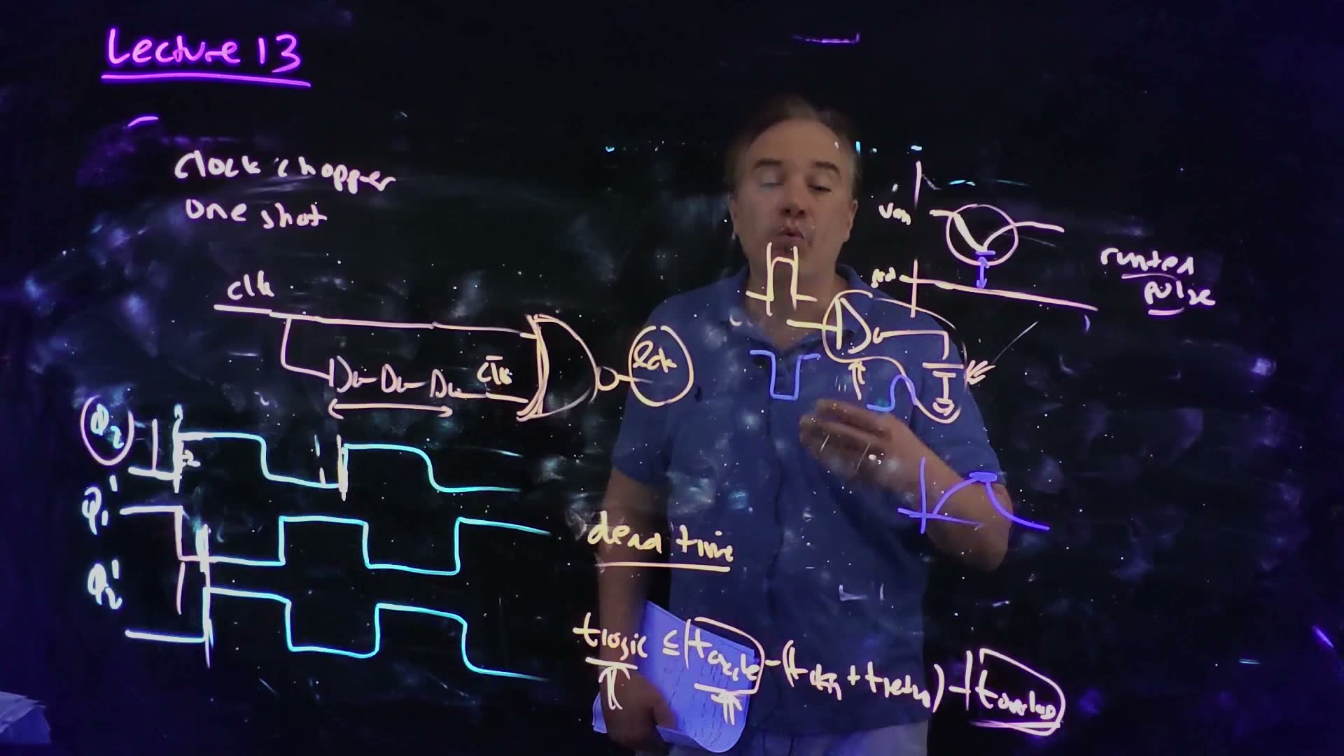
Fair copy of the board above (Lecture13 @ 38:00), mark for mark in its own layout. Since 34:41 the clk, clk̄ and lclk waveforms at the right have been erased, and lclk at the chopper’s output has been circled (35:24); the chopper, the φ rows, “dead time” and the long-path inequality are kept. Black is the cyan pen (the φ2, φ1′ and φ2′ rows and their labels) and the purple pen (the title and the circle round φ2). Orange is the orange pen: the chopper and the kept marks, and the new runted-pulse sketch with “runted pulse” (pale yellow at its left, pink to lavender to the right; one pen). Blue is a blue pen, a separate layer: the negative input pulse, the bump under the inverter, the arrow from the dip towards gnd, and the output at the bottom that rises only part way. The lecturer draws the inverter as a D; it is drawn here as a triangle.

How tall is a runt?

The lecture draws the runt without numbers. A first-order estimate needs only the course’s 50%-point delay added. Model the driver’s output as an RC circuit driven by a step: from 0, it reaches the fraction $1 - e^{-t/\tau_{RC}}$ of its swing after a time $t$t.

The runt's height (added)

1. Calibrate the RC to the course’s delay. The driver’s delay $t_d$ is the time to reach 50%: $1 - e^{-t_d/\tau_{RC}} = \tfrac12$21​, so $\tau_{RC} = t_d/\ln 2$td​/ln2.
2. Stop the charging at the end of the pulse. The output moves for $t_{pulse}$tpulse​, then turns back. Its peak, as a fraction of $V_{DD}$VDD​, is $1 - e^{-t_{pulse}/\tau_{RC}} = 1 - e^{-(t_{pulse}/t_d)\ln 2} = 1 - 2^{-t_{pulse}/t_d}$2−tpulse​/td​.
3. Read it. A pulse as wide as the driver’s delay just reaches $V_{DD}/2$VDD​/2. A narrower pulse never crosses the middle of the swing, so the latch’s own clock buffer may not switch at all.

How tall a pulse gets through a driver of 50% delay $t_d$ added, computed from the first-order model $v/V_{DD} = 1 - 2^{-t/t_d}$ while the pulse lasts and an exponential decay after it. A pulse as long as $t_d$ just reaches $V_{DD}/2$VDD​/2; one half as long reaches only $0.29\,V_{DD}$0.29VDD​, a runt the next gate may not see at all; one twice as long reaches $0.75\,V_{DD}$0.75VDD​.

The height of a pulse through a slow driveradded

$$\frac{v_{peak}}{V_{DD}} = 1 - 2^{-t_{pulse}/t_d}$$

Holds when: the driver's output modelled as a first-order RC driven by a step from rest; t_d is its 50% delay into this load (Chapter 7's definition), so τ_RC = t_d/ln 2; the driver's own parasitic ignored

Memorize or derive. Memorize the rule: the pulse must be wider than the delay of whatever drives it, or it does not reach half the swing. Derive the height when a question asks for it, in three steps: the RC charge $1 - e^{-t/\tau_{RC}}$e−t/τRC​, $\tau_{RC} = t_d/\ln 2$ from the 50% definition, then substitute $t = t_{pulse}$tpulse​. State the convention you use: a paper that calls $t_d$ the RC time constant itself would get $1 - e^{-t_{pulse}/t_d}$e−tpulse​/td​, a taller runt. This guide keeps Chapter 7’s 50%-point delay, which Chapter 7 warns not to multiply by $\ln 2$ a second time.

A worked example

An added example added: a driver whose FO1 delay is 20 ps drives a load 10 times its own input capacitance.

Three pulses through one driver

1. The driver’s delay into this load. $t_d = 20 \times 10 = 200$ ps, and $\tau_{RC} = 200/\ln 2 = 289$ ps.
2. A 100 ps pulse. $1 - 2^{-100/200} = 1 - 2^{-0.5} = 0.29$0.29: the output moves only 29% of the swing. A runt.
3. A 200 ps pulse reaches $1 - 2^{-1} = 0.50\,V_{DD}$0.50VDD​, just half; a 400 ps pulse $1 - 2^{-2} = 0.75\,V_{DD}$0.75VDD​.

Traps.

• Using $t_d$ itself as $\tau_{RC}$τRC​. That is the other convention; with the course’s 50% delay it double-counts $\ln 2$ and gives a taller runt than the model predicts.
• Widening the pulse to beat the runt without re-checking hold. Section 4’s constraint, $t_{logic} \ge t_{skew} + t_{pulse} + t_{hold} - t_{clk\to Q}$tclk→Q​, caps the width.
• Thinking a runt only delays the latch. It may never open it.

Check yourself Why does a chopper inside every flip-flop avoid runts?

Its pulse goes straight to the latch it opens, through no long wire and no driver with a large load, so the pulse’s width is far larger than the delay of anything it passes through.

Check yourself Hold caps the pulse at 60 ps. A driver has an FO1 delay of 15 ps. What is the largest load, as a multiple of its input capacitance, for which the pulse still reaches V_DD/2? How tall is the pulse at a ratio of 8?

The pulse reaches half the swing when $t_d \le t_{pulse}$tpulse​: $15 \times k \le 60$60, so $k \le 4$4. At $k = 8$8, $t_d = 120$ ps and the peak is $1 - 2^{-60/120} = 0.29\,V_{DD}$0.29VDD​.

Check yourself What does a runt pulse mean for the latch it clocks?

The latch’s clock may never cross its switching threshold, so the latch may never open, or open weakly and late; the data it should have taken is lost.

7. Transparent-latch design and cycle stealing

You need

A flip-flop is two latches (Chapter 13; Section 3 here). A master latch on φ1 followed at once by a slave latch on φ2, with nothing between them. φ1 and φ2 are complementary phases: φ1 high in the first half of each cycle, φ2 in the second.

The flip-flop pair as four latches, φ1 φ2 | logic | φ1′ φ2′ (Lecture13 @ 24:39, redrawn). Here only the circuit matters: each flip-flop is a φ1 latch touching a φ2 latch. Original figure ↑

Transparency (Chapter 13). Data that reaches a latch while the latch is open passes straight through, after the latch’s D-to-Q delay. This section, like the lecture, takes that delay as zero.

The flip-flop long path (Section 1). Each stage between two flip-flops gets exactly one cycle, minus the overhead: $t_{logic} \le T_{cycle} - (t_{clk\to Q} + t_{setup})$tsetup​). The slowest stage sets the clock.

The question. Flip-flop design gives every stage exactly one cycle, no more and no less. What if one stage needs more and its neighbour less?

The weakness of flip-flop design

Flip-flop timing is simple, and the lecturer gives it its due (38:40–42:30). Every pair of flip-flops can be checked on its own, for the long path and for the short path, so the analysis is local. Its weakness is the same rigidity: optimal design needs exactly one cycle of logic in every stage, and the partition into stages propagates all the way up into the RTL. If the logic is partitioned poorly, the slowest stage sets the clock and every other stage waits. That is part of why, in the lecturer’s numbers, a typical ASIC runs at 300–500 MHz with long paths of about 50 FO4, while a microprocessor in the same technology runs at about 3 GHz. And even a good partition is unbalanced again by PVT variation, which slows some paths more than others.

Separate the master from the slave

From flip-flops to separated latches (board, 42:30–45:30)

1. Write each flip-flop as its two latches (42:15) board: φ1 then φ2, touching.
2. Separate them (43:00) board: move part of the logic in between, so there is logic between every pair of latches, and the phases alternate φ1, φ2, φ1, φ2 along the path. The board calls this transparent, or separated, latch design. The alternation is what keeps the flip-flop design’s sequencing: no data can pass two latches of the same phase in one half cycle.
3. The blocks need not be equal (44:51) board. A long block that is still running when the next latch opens simply finishes during that latch’s transparent phase, and the data flows straight through. The slow block has borrowed time from the next one: cycle stealing (the lecturer’s term; “time borrowing” is another name for it). While the rules of Section 8 hold, nothing waits for a clock edge, so there is no dead time.

Two ways to use the same latches, redrawn from the board (Lecture13 @ 46:28). Top: each φ1/φ2 pair sits back to back and acts as a flip-flop, with all the logic between flip-flops. Bottom: transparent (separated) latch design spreads the logic between every pair of latches, so a slow block can borrow time from the next half cycle: cycle stealing.

The board (Lecture13 @ 46:28)

Lecture13 @ 46:28Flip-flops (top) separated into latches with logic between every pair (bottom): cycle stealing.

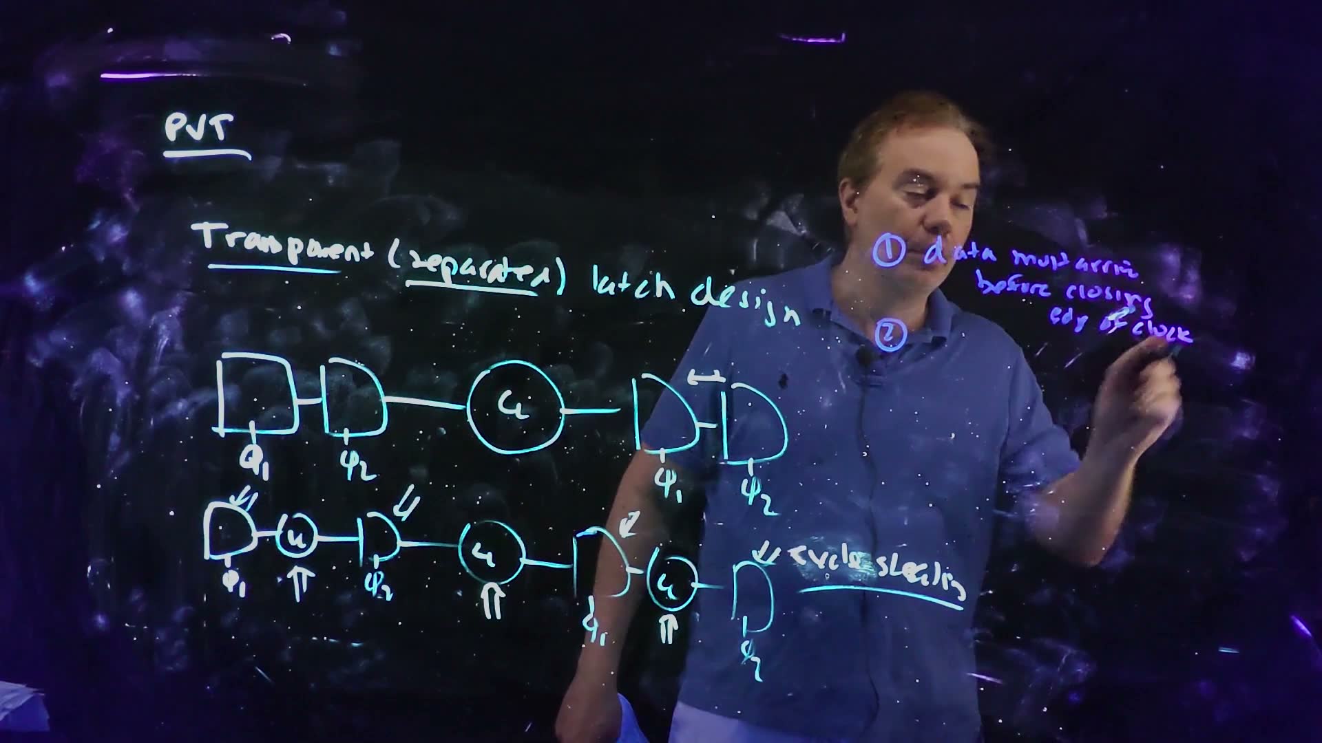
Fair copy of the board above (Lecture13 @ 46:28), mark for mark in its own layout. The runt-pulse board has been erased; only the purple remnants at the top are left (the old title’s underline, a stroke of its “3” and the dash). Black is the cyan pen: “PVT”, the title, both rows of latches and logic with their labels and arrows, and “cycle stealing”. Blue is the blue pen, a separate layer: the circled 1 with rule 1 and the circled 2, whose rule follows by 48:51. The lecturer draws the latches as D shapes; they are copied as drawn.

What borrowing buys

An added example added, with every overhead and latch delay ignored. Two stages of logic, 1000 ps in all, split unevenly: 600 ps and 400 ps.

Flip-flops against separated latches (added)

1. With flip-flops. Each stage must fit in one cycle, so the clock must accommodate the 600 ps stage: $T_{cycle} = 600$ ps. The 400 ps stage then idles for 200 ps every cycle.
2. With separated latches, the same logic as four blocks, 300, 300, 200 and 200 ps, between φ1, φ2, φ1, φ2 latches, at $T_{cycle} = 500$ ps. φ1 is open on 0–250 ps, 500–750 ps and from 1000 ps; φ2 on 250–500 ps and 750–1000 ps.
3. Walk the data. Launched at 0, it reaches the first φ2 latch at 300 ps (open: it passes), the next φ1 latch at 600 ps (open 500–750: it passes), the next φ2 latch at 800 ps (open 750–1000) and the φ1 latch after that at 1000 ps, just as it opens. Nothing ever waited.
4. The gain. The cycle is 500 ps instead of 600 ps: 17% shorter, so the clock is 20% faster, from the same logic.

Flip-flops against separated latches added, computed from two logic blocks of 600 ps and 400 ps with overheads ignored. With flip-flops (top), every cycle must hold the slower block: $T_{cycle} = 600$ ps, and the 400 ps block leaves 200 ps idle (hatched), 1200 ps for both. With two-phase latches (bottom), $T_{cycle} = 500$ ps: the same logic as blocks of 300, 300, 200 and 200 ps reaches each latch while it is open, at 300, 600, 800 and 1000 ps, and both stages finish in 1000 ps.

Traps.

• Two latches of the same phase in a row. Then data can pass both in one half cycle, and the one-step-per-cycle sequencing is lost. The phases must alternate.
• Thinking latch design needs no timing check. It needs a different one, and it is no longer local: that is Section 8.

Check yourself Why must the phases alternate φ1, φ2, φ1, φ2?

At any moment only one phase is high. With alternating phases, data that passes an open latch then meets a closed one, so it advances by one latch per half cycle, two per cycle: the same sequencing as one flip-flop per cycle. Two open latches of the same phase in a row would let it run through both at once.

Check yourself Two stages need 700 ps and 300 ps. What clock period do flip-flops need? What could separated latches reach, with latch delays ignored, and what must be true of the blocks?

Flip-flops need 700 ps, the slower stage. Separated latches could reach 500 ps, since the total is 1000 ps over two cycles, provided the 700 ps stage is split so that every arrival comes before its latch’s closing edge: for example 350, 350, 150 and 150 ps, which arrive at 350, 700, 850 and 1000 ps, each inside its latch’s open phase.

Check yourself Name two reasons the lecturer gives for stages being unbalanced in a flip-flop design.

A poor partition of the logic into cycles, which then propagates into the RTL; and PVT variation, which changes some paths’ delays more than others even when the partition was good.

8. The two rules of the road and static timing

You need

Separated latches (Section 7). Logic sits between every pair of latches, and the latches alternate φ1, φ2, φ1, φ2. A slow block may finish while the next latch is open, and the data passes straight through: cycle stealing.

Flip-flops against separated latches (Lecture13 @ 46:28, redrawn): in the bottom row there is logic between every pair of latches. Original figure ↑

The closing edge (Chapter 13). A transparent-high latch closes on its clock’s falling edge; data that arrives after that is held back until the latch opens again, a cycle late. As the lecture draws them, φ1 is high in the first half of each cycle and φ2 in the second.

The lecture’s simplifications. Setup time, hold time and the latches’ own delays are taken as zero in this section and the next.

The question. Flip-flop design is checked one pair at a time. With separated latches, a block may borrow from the next, which may borrow from the next. What has to be true for all that borrowing to work, and how does anyone check it on a chip with millions of latches?

The two rules

Rules of the road (board, 45:30–48:50)

1. Rule 1: data must arrive before the closing edge of every latch (45:42) board. With a setup time, $t_{setup}$ before it (46:59). This is the flip-flop’s setup rule, except that it is now checked at every latch, master and slave alike, because each one can be where a borrowed block finishes.
2. Rule 2: whenever a loop closes, the delay in the loop must be at most the number of cycles in the loop (47:13) board. A loop is any path that comes back to a latch it started from: the separated chain of Section 7, closed by logic back to its first latch.
3. Counting the cycles added. In an alternating φ1/φ2 loop, every two latches are one cycle, so the loop has half as many cycles as latches. A flip-flop’s output fed back to its own input (two latches) is a one-cycle loop; the four-latch loops of Section 9 are two cycles. The lecturer’s spoken example: a loop of a thousand cycles must have less than a thousand cycles of delay.

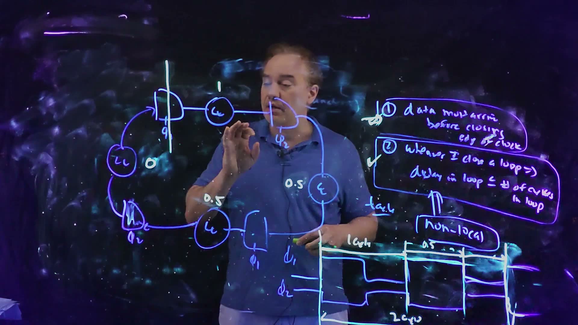
Closing the separated-latch chain into a loop, redrawn from the board (Lecture13 @ 50:51). Time borrowed by one block must be repaid somewhere around the loop, so the loop as a whole must fit its delay into the number of cycles it contains: this four-latch loop has two.

The board (Lecture13 @ 50:51)

Lecture13 @ 50:51The chain closed into a loop, the two rules of the road, and STA.

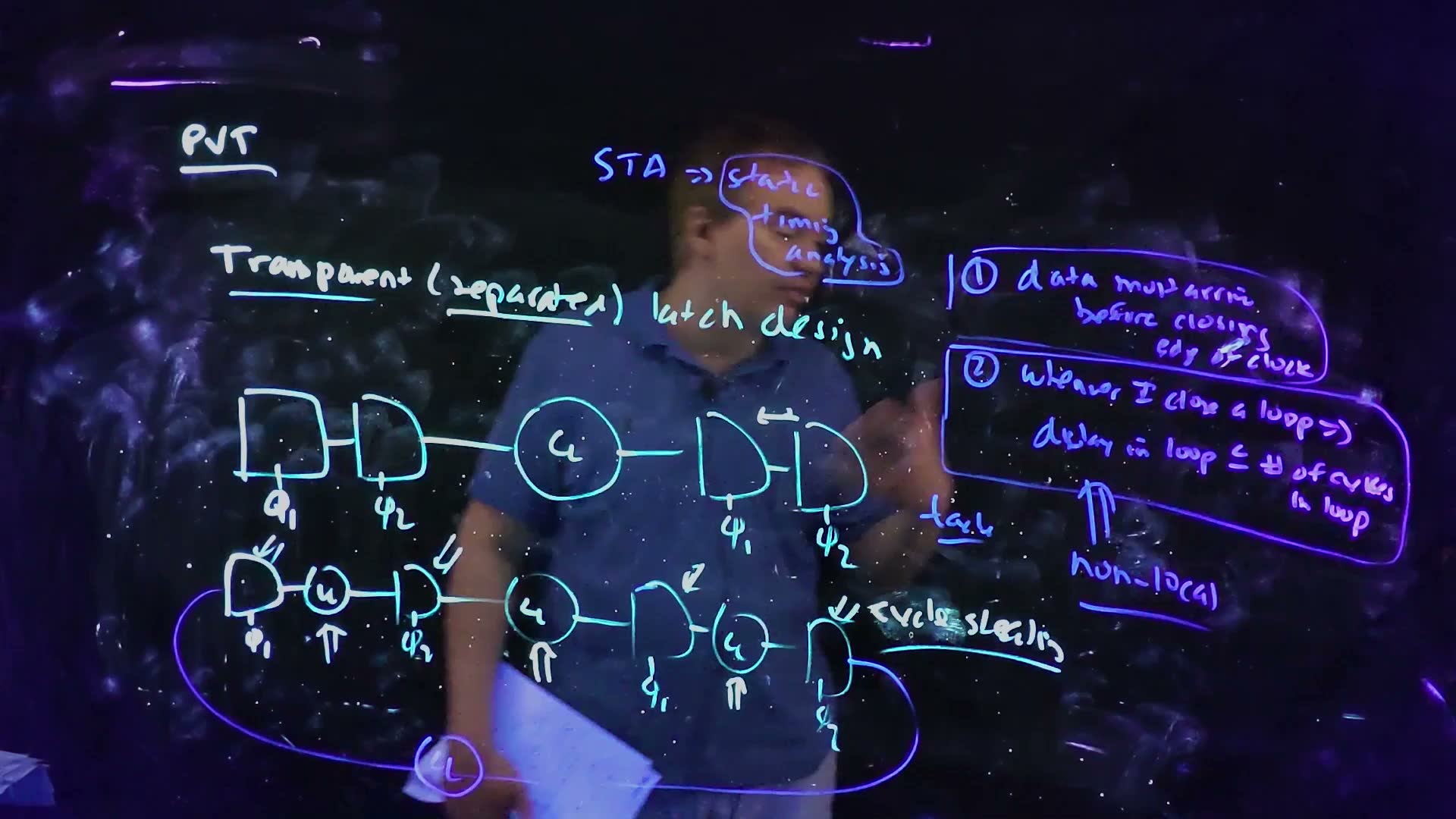
Fair copy of the board above (Lecture13 @ 50:51), mark for mark in its own layout. The 46:28 board is kept as it was. Black is the cyan pen (PVT, the title, both rows and “cycle stealing”) and the purple remnants at the top. Blue is the blue pen: rule 1 from before, and everything new: “STA ⇒ static timing analysis” with a cloud round its words, the boxes round both rules, rule 2, the double arrow to “non-local”, $t_{cycle}$tcycle​, and the wire that closes the bottom row into a loop through a third $C_L$CL​. “STA” and $t_{cycle}$ look paler than the rules but measure as the blue pen. The circled $C_L$ on the loop is half hidden by the lecturer’s papers at 50:51 and is read from 50:06, where it is unchanged.

Why rule 2 is the hard one

Rule 2 is non-local (48:36) board. A chain of 10,000 latches can borrow time down its length with every local check passing, until the last block closes the loop. Then the violation appears, and fixing it may mean re-examining 10,000 cycles of logic. This, the lecturer says, is why latch design is less common than it should be: its timing is not a property of any one pair of latches.

Why is rule 2 needed at all, if rule 1 is checked at every latch added? Because rule 1 is checked against arrival times, and each arrival depends on when the data left the latch before. Around a loop, a block that runs a little long makes the next lap start a little late; if the loop holds more delay than it has cycles, that lateness grows every lap, until some arrival misses a closing edge, perhaps many cycles later. Rule 2 is the steady-state version of that walk. Section 9 shows a loop that passes rule 1 on its first lap and fails it on the second.

Static timing analysis

This is the job of static timing analysis (STA) (48:50–51:17) board. An STA tool traces the longest paths through the combinational logic and compares their delays with the constraints set by the clocked elements: rule 1 at each latch, and the loops for rule 2. “Static” means it uses no test patterns and runs no simulation: it adds delays along paths. The price is that it may report a false path (49:43), a path through the logic that no input can actually exercise, so a designer must judge whether a reported violation is real. Section 9 shows how STA handles a loop whose first lap seems to fail: it moves the launch point (Lecture 14, 06:06).

Rule 1board

$$\text{arrival at each latch} \le \text{its closing edge} - t_{setup}$$

Holds when: every transparent latch, master or slave; setup and hold zero as in the lecture; the board writes it without setup, and the setup term is spoken (46:59): with setup, t_setup before the closing edge

Rule 2board

$$\sum_{\text{loop}} t_{logic} \le N_{cycles}\, T_{cycle}$$

Holds when: every loop of latches; for alternating φ1/φ2 latches the loop's cycle count is half its number of latches (the counting is added); latches add no delay

Memorize or derive. Memorize both rules; they are what the exam’s latch questions check. Derive the consequence that no single block between two latches may take more than one cycle: Section 9’s second example derives it from rule 1.

Traps.

• Counting latches instead of cycles. Four alternating latches are two cycles, not four.
• Checking rule 1 against the opening edge. Arriving after the opening edge is fine, that is cycle stealing; the deadline is the closing edge.
• Thinking STA proves the design works. It checks timing, not function, and it may flag false paths.

Check yourself A loop of six alternating latches holds 2.7 cycles of logic in total. Does rule 2 hold?

Six alternating latches are three cycles, and $2.7 \le 3$3: yes. (Rule 1 must still be checked at each latch.)

Check yourself A loop φ1 → [7 ns] → φ2 → [4 ns] → φ1 → [6 ns] → φ2 → [5 ns] → back to the first φ1, clocked at T_cycle = 10 ns with no skew. Does rule 2 hold? If not, what is the smallest period rule 2 allows, and does rule 1 then hold everywhere?

The loop has $7 + 4 + 6 + 5 = 22$ ns of delay and two cycles, 20 ns: rule 2 fails. It needs $2T_{cycle} \ge 22$ ns, so $T_{cycle} \ge 11$ ns. At 11 ns, φ1 is open on 0–5.5 ns and φ2 on 5.5–11 ns, and so on. Launched at 0, the data reaches the φ2 latch at 7 ns (open until 11), the φ1 latch at 11 ns (just opening), the next φ2 latch at 17 ns (open 16.5–22) and the first latch at 22 ns (just opening). Rule 1 holds at every latch.

Check yourself Why is rule 2 called non-local?

A loop can run through thousands of latches. Every local check can pass along the way, and the violation shows up only when the whole loop is added up; finding and fixing it may involve every block in the loop.

9. Worked examples: four-latch loops

You need

The two rules of the road (Section 8). Rule 1: data must arrive before the closing edge of every latch. Rule 2: around every loop, the total delay must be at most the number of cycles in the loop; an alternating φ1/φ2 loop of four latches holds two cycles.

A separated-latch chain closed into a loop (Lecture13 @ 50:51, redrawn): four alternating latches, two cycles. Original figure ↑

The clocks. As the lecture draws them, φ1 is high on $[0, \tfrac12)$ of each cycle and φ2 on $[\tfrac12, 1)$[21​,1): complementary, with no non-overlap. Every latch is transparent while its clock is high and closes on its clock’s falling edge. So a φ1 latch is open from $k$ to $k + \tfrac12$ and a φ2 latch from $k + \tfrac12$ to $k + 1$1, for each whole number $k$k. Times and delays are in clock cycles.

What a latch does with arriving data. If the data arrives while the latch is open, it passes at once (the latches add no delay here). If it arrives while the latch is closed, it waits for the opening edge; that wait is dead time. If it arrives after the closing edge it was meant for, rule 1 is broken.

The launch assumption (53:28). The walk starts at a φ1 latch, launched on φ1’s rising edge, $t = 0$0. Example 3 shows why that assumption can mislead.

The question. Given the four delays of a φ1/φ2 loop, does it work? The method is the lecture’s: walk the data around the loop, edge by edge, and check rule 1 at every latch and rule 2 at the end.

The arrival walkadded

$$\text{leave}_k = \max(\text{arrive}_k,\ \text{open}_k)$$$$\text{arrive}_{k+1} = \text{leave}_k + d_k$$$$\text{rule 1: } \text{arrive}_k \le \text{close}_k$$

Holds when: transparent-high latches on φ1 and φ2; setup, hold and latch delays zero; arrive_k, open_k and close_k are the arrival and the window at the k-th latch visited, d_k the logic after it

This is rule 1 written as arithmetic: wait for the latch if it is closed, then add the next block’s delay. The lecture does exactly this on the board, with arrows. Memorize or derive. Derive it each time from what a transparent latch does; there is nothing to memorize beyond rule 1.

Example 1: cycle stealing with no dead time

The loop (51:00) board: φ1 → 0.75 → φ2 → 0.25 → φ1 → 0.75 → φ2 → 0.25 → back to the first φ1. Call the latches L1 to L4 in that order.

Latch loop, example 1, redrawn from the board (Lecture13 @ 52:51). Four latches alternate φ1, φ2, φ1, φ2 around a ring, with logic between each pair; the numbers are the logic delays in clock cycles (0.75, 0.25, 0.75, 0.25), and the data flows clockwise. The loop holds four latches, so it spans two cycles. The board writes “C_L” (combinational logic) in each circle; the redraw writes the delay there.

The board (Lecture13 @ 52:51)

Lecture13 @ 52:51Example 1's loop beside the two rules of the road: φ1, φ2, φ1, φ2 with 0.75 (top, hidden here), 0.25, 0.75 and 0.25.

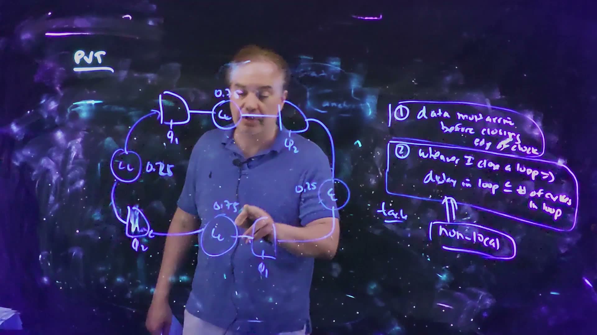
Fair copy of the board above (Lecture13 @ 52:51), mark for mark in its own layout. The rules, “non-local” and $t_{cycle}$ are kept from 50:51; the latch rows, STA and the loop wire are erased, and “non-local” now has a box round it. Black is the cyan pen (PVT) and the purple remnants at the top. Blue is the blue pen: the rules, and the new ring of four latches, φ1, φ2, φ1, φ2 clockwise from the top left, with a $C_L$ between each pair and the delays 0.25 (left), 0.25 (right) and 0.75 (bottom). The $C_L$ at the right is written as a squeezed C over L and looks like ε. The top delay is behind the lecturer’s head: only “0.” and one stroke of the next digit show, and they are copied as they stand. At 52:06 his face hides it as well, and by 55:30 it has been rubbed out and replaced by 1. He says “three quarters of a cycle” as he writes it (51:51), and the walk at 55:30 starts with 0.75.

Walking example 1 (board, 51:51–55:01)

1. Launch. The data leaves L1 when φ1 rises, at $t = 0$0.
2. L2 (φ2, open ½ to 1). It arrives at $0 + 0.75 = 0.75$0.75. φ2 is open, so the data passes at once. Rule 1: $0.75 < 1$1.
3. L3 (φ1, open 1 to 1½). It arrives at $0.75 + 0.25 = 1.0$1.0, just as φ1 opens: it passes, without waiting.
4. L4 (φ2, open 1½ to 2). It arrives at $1.0 + 0.75 = 1.75$1.75; open; $1.75 < 2$2.
5. Back to L1 (φ1, opens at 2). It arrives at $1.75 + 0.25 = 2.0$2.0, as φ1 opens: the next lap starts exactly where the first one did, two cycles later.
6. Rule 2. The loop’s delay is $0.75 + 0.25 + 0.75 + 0.25 = 2.0$2.0, against 2 cycles: it fits, exactly. “I have never waited”: every arrival found its latch open or opening, so there is no dead time, and each 0.75 block borrowed a quarter cycle from the 0.25 block after it.

Walking example 1 around the loop, times in clock cycles (redrawn from the board, Lecture13 @ 55:30). Launched when φ1 opens at 0, the data reaches the φ2 latch at 0.75 (open, so it passes straight through), the next φ1 latch at 1.0 (just as it opens), the second φ2 latch at 1.75, and the first latch again at 2.0. Every arrival comes before its latch’s closing edge, and the loop closes in exactly 2 cycles, with no waiting.

The board (Lecture13 @ 55:30)

Lecture13 @ 55:30Example 1's walk: 0.75, 0.25, 0.75, 0.25 over φ1 and φ2, closing in 2 cycles. The ring's top label already reads 1, the start of example 2.

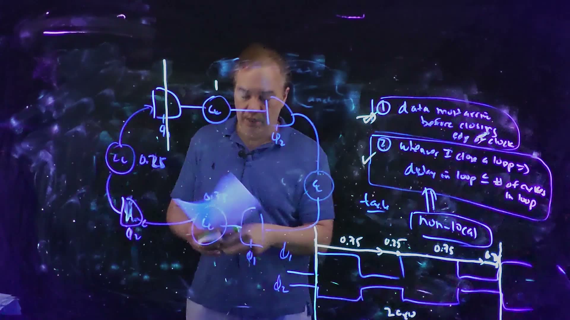
Fair copy of the board above (Lecture13 @ 55:30), mark for mark in its own layout. The ring and the rules are kept from 52:51; PVT, the right delay and the top delay are rubbed out, and a 1 now stands at the top, the start of example 2. The bottom delay, 0.75, is partly behind the lecturer’s papers here and is copied whole, as at 52:51. Black is the cyan pen, which looks white on this board: the vertical line through the first φ1 latch, the 1, a scribbled mark by rule 1 and a check mark by rule 2, and the walk’s two time axes, the arrow along the top with the labels 0.75, 0.25, 0.75 and 0.2†, and “2 cycles”. Blue is the blue pen: the ring, the rules, and φ1 and φ2 with their waveforms, which turn violet past the right axis, at the edge of the view; it is one pen. φ1’s high from 1 to 1.5 cycles lies under the arrow. †The last label is squeezed against the axis and reads 0.2; the delay is 0.25 (“I get another 0.25 here”, 54:31).

Example 2: arriving in the nick of time

The same loop with delays 1, 0.5, 0.5 and 0 (55:26) board.

Latch loop, example 2, redrawn from the board (Lecture13 @ 58:00): the same ring with logic delays of 1, 0.5, 0.5 and 0 cycles. The loop’s total is still 2 cycles, but now one block takes a whole cycle.

Walking example 2 (board, 55:26–57:39)

1. L2 (φ2, open ½ to 1). The data leaves L1 at 0 and arrives at $0 + 1 = 1.0$1.0: exactly as φ2 closes. Rule 1 asks for arrival before the closing edge; with setup taken as zero, arriving on it meets the rule with equality. It works, but with nothing to spare.
2. L3 (φ1, open 1 to 1½). It arrives at $1.0 + 0.5 = 1.5$1.5, again as φ1 closes: “just in the nick of time” (57:06).
3. L4 (φ2, open 1½ to 2). $1.5 + 0.5 = 2.0$2.0, as φ2 closes.
4. Back to L1. $2.0 + 0 = 2.0$2.0, as φ1 opens. The loop’s delay is $1 + 0.5 + 0.5 + 0 = 2.0 \le 2$ cycles: “this also will work” (57:39).

Walking example 2, times in cycles (redrawn from the board, Lecture13 @ 58:00). The 1-cycle block delivers its data to the φ2 latch at 1.0, exactly as φ2 closes; the next two blocks deliver at 1.5 (φ1 closing) and 2.0 (φ2 closing); the zero-delay block hands it to the first latch at 2.0, just as φ1 opens. Each of the first three arrivals meets rule 1 with equality, and the loop still closes in 2 cycles.

The board (Lecture13 @ 58:00)

Lecture13 @ 58:00Example 2: delays 1, 0.5, 0.5 and 0; the walk ends on a closing edge three times and closes in 2 cycles.

Fair copy of the board above (Lecture13 @ 58:00), mark for mark in its own layout: example 2 on the ring of example 1. The ring, the rules, the line through the first latch, the marks by the rules, the time axes and φ1 and φ2 are kept from 55:30. Black is the cyan pen: the delays 1 (top, already there at 55:30), 0.5 (right), 0.5 (bottom) and 0 (left), the lines at 1 and 1.5 cycles, the arrow along the top (its first piece kept; its heads and the rest drawn again), “1 cycle” and 0.5, and an arrow back along the bottom to the left axis, which runs off the bottom of the view. Blue is the blue pen. The walk’s old labels and the old arrow beyond 1 cycle were rubbed out and leave a haze along the top, which is not copied.

The lesson (spoken, 56:47). Look at step 1. A block launched when its latch opens has until the next latch closes, and with complementary phases that is exactly one cycle later. So no block between two latches may take more than one cycle: “if it’s more than this, I would have a violation”. A half-cycle phase can lend its whole time to the block before it, but no more.

One block, at most one cycle

$$d_k \le T_{cycle}$$

Holds when: spoken (56:47); complementary φ1/φ2 latches, setup and latch delays zero; the block's data leaves its latch no earlier than the latch's opening edge

Memorize or derive. Derive it in two lines: the data cannot leave latch $k$ before latch $k$ opens; latch $k + 1$ closes one cycle after that. So a block longer than a cycle misses the closing edge, whatever the other blocks do.

What breaks a loop

Two added loops added, each with a total that looks harmless, show why both rules are needed.

Two failures (added)

1. Rule 2 holds, rule 1 fails: 1.25, 0.25, 0.25, 0.25. The total is 2.0, within 2 cycles. But the first block alone is 1.25 cycles: launched at 0, the data reaches L2 at 1.25, after φ2 closed at 1.0. Rule 1 fails, as the one-cycle limit says it must.
2. Rule 1 holds on lap 1, rule 2 fails: 0.75, 0.5, 0.75, 0.25. The total is 2.25, more than 2 cycles. Lap 1: L2 at 0.75 (open), L3 at 1.25 (open 1 to 1½), L4 at 2.0 (exactly as φ2 closes), L1 at 2.25 (open 2 to 2½, so it passes). Every arrival met rule 1. But lap 2 starts at 2.25, a quarter cycle late: L2 at 3.0 (exactly as φ2 closes), L3 at 3.5 (exactly as φ1 closes), and L4 at 4.25, after φ2 closed at 4.0. Rule 1 fails on the second lap. A loop that holds too much delay loses its excess every lap until an arrival misses its edge; that is what rule 2 prevents.

Example 3: dead time, and moving the launch point

Lecture 14 opens with a third loop (L14 01:08) board: φ1 L1 → 0.25 → φ2 L2 → 1.0 → φ1 L3 → 0.5 → φ2 L4 → 0.25 → back to L1. The total is $0.25 + 1.0 + 0.5 + 0.25 = 2.0$2.0: two cycles, exactly.

Latch example 3, redrawn from the board (Lecture14 @ 06:26): the same four-latch ring as Lecture 13’s examples, with logic delays of 0.25, 1.0, 0.5 and 0.25 cycles. The total is 2 cycles, as the loop allows, but the first block is short. The dashed line through the first latch marks where the loop is cut to start the walk.

Walking example 3 (board, Lecture14 01:50–06:32)

1. Launch on φ1’s rising edge, as before (02:29). The data reaches L2 at 0.25, but L2’s φ2 does not open until 0.5. “So there is a dead time”: the data waits a quarter cycle for L2 to open (02:56).
2. The rest of the lap. It leaves L2 at 0.5 and reaches L3 at $0.5 + 1.0 = 1.5$1.5, exactly as φ1 closes; L4 at $1.5 + 0.5 = 2.0$2.0, exactly as φ2 closes; and L1 at $2.0 + 0.25 = 2.25$2.25, while φ1 is open (2 to 2½). Rule 1 holds at every latch.
3. But the lap took 2.25 cycles (04:09). Measured from the launch at 0, the data is back at L1 at 2.25: a quarter cycle over the loop’s two cycles, because of the dead time. At first glance rule 2 is violated.
4. The launch assumption is the problem (04:20). Nothing says the data must leave L1 on φ1’s rising edge. L1 is transparent for the whole half cycle, so the data “could have arrived anywhere in the transparency window of φ1, and that would have been just fine” (04:47).
5. Walk the launch forward (04:52–05:37). Launch at 0.25 instead. The data reaches L2 at 0.5, exactly as it opens: no dead time. Then L3 at 1.5, L4 at 2.0 and L1 at 2.25, which is $0.25 + 2$2: the lap takes exactly two cycles, and the next lap starts at the same point of the cycle. Rule 2 holds, and the loop works.
6. What STA does (06:06–06:32). A static timing tool does the same: it breaks the loop, finds the apparent violation, and walks the launch edge forward in small steps. If the return can be made to meet the launch in the right number of cycles, there is no violation; if not, there is.

Walking example 3 from φ1’s opening edge, times in cycles (redrawn from the board, Lecture14 @ 04:26). The first block delivers its data at 0.25, but the φ2 latch is closed until 0.5: the data waits (hatched: dead time). The next blocks take 1.0, 0.5 and 0.25, arriving at 1.5 and 2.0 exactly on closing edges and back at 2.25. The wait makes the lap look like 2.25 cycles, although the loop holds only 2 cycles of delay.

The board (Lecture14 @ 04:26)

Lecture14 @ 04:26Example 3 launched on φ1's rising edge: the hatched dead time at L2, and rule 2 crossed out at first.

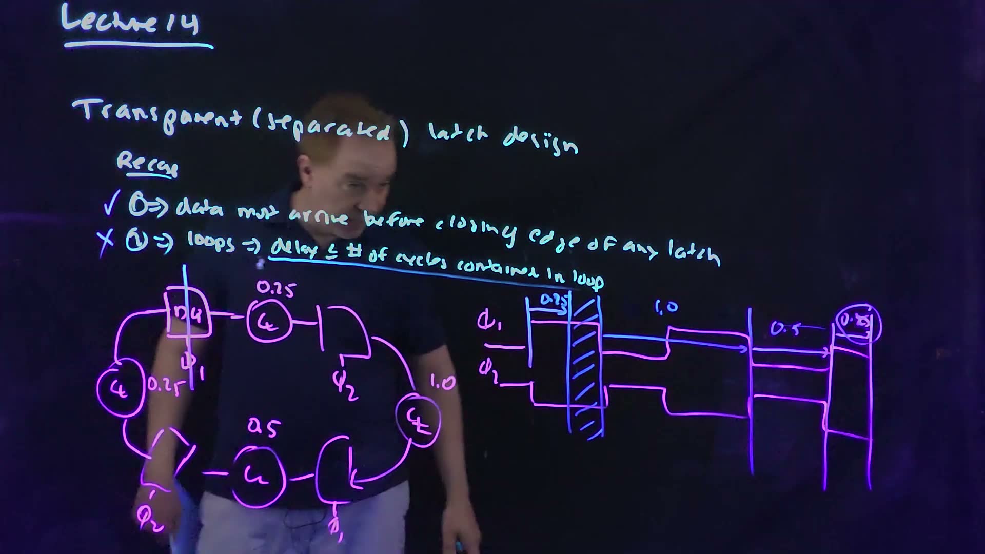
Fair copy of the board above (Lecture14 @ 04:26), mark for mark in its own layout: the recap of the two rules, and example 3 walked from φ1’s rising edge. Black is the cyan pen, which reads white: the title, “Recap”, rule 1 (data must arrive before closing edge of any latch) and rule 2 (loops ⇒ delay ≤ # of cycles contained in loop) with its underline. Magenta is the pink pen: the ring of four latches, φ1, φ2, φ1, φ2 clockwise from the top left, with a $C_L$ between each pair and the delays 0.25 (top), 1.0 (right), 0.5 (bottom) and 0.25 (left), and φ1 and φ2 with their waveforms at the right. Blue is the blue pen: the check by rule 1 and the cross by rule 2, the break line through the first φ1 latch, and the walk: the time guides, the 0.25 arrow from the launch at 0, the hatched dead time from 0.25 to 0.5, the arrows 1.0 and 0.5, and the circled 0.25 at the end. Towards the right edge of the view the blue pen turns violet; it is one pen. The marks inside the first latch are copied as they stand, and its φ1 is set just right of the break line, which runs through it on the board. The lecturer stands in front of the middle of the board here; the ring’s right half and the middle of the rules are read from 06:26 and 07:07, where they are unchanged.

The same loop walked the way static timing analysis does it (redrawn from the board, Lecture14 @ 06:26): start when the data actually leaves the first latch, at 0.25. It reaches the φ2 latch just as it opens at 0.5, meets the closing edges at 1.5 and 2.0, and returns at 2.25, exactly 2 cycles after it left. The dead time of the edge launch came from choosing the wrong starting point.

The board (Lecture14 @ 06:26)

Lecture14 @ 06:26The launch walked forward to 0.25: the loop closes in 2 cycles, and rule 2 is checked. 'STA' above: this is how a timing tool checks it.

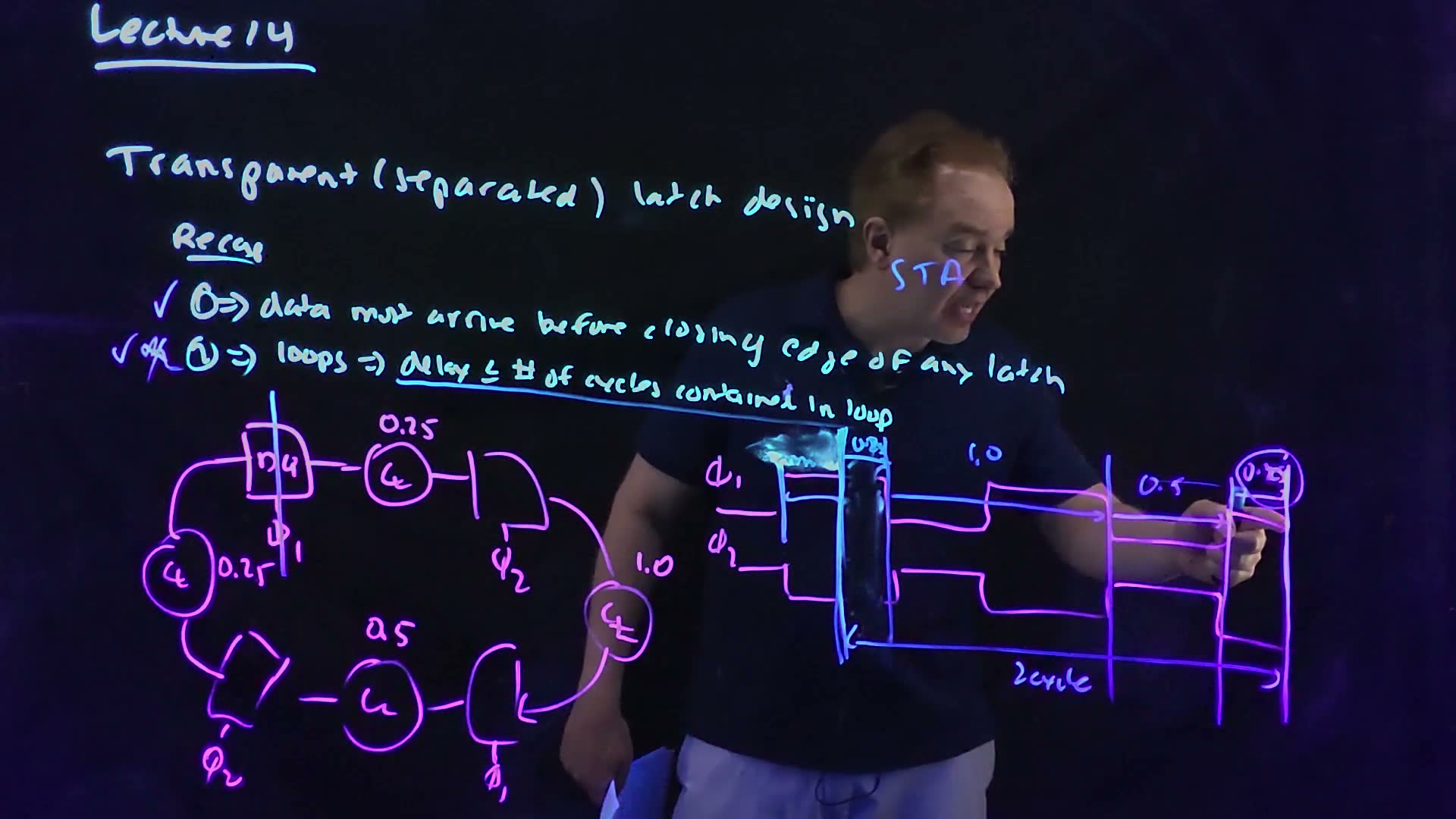
Fair copy of the board above (Lecture14 @ 06:26), mark for mark in its own layout: example 3 with the launch walked forward to 0.25. The title, the rules, the ring and the clocks are kept from 04:26. Rubbed out since then: the hatched dead time, the first 0.25 label and its arrow from 0, and the pieces of φ1’s high and φ2’s low under the hatching; the haze the eraser leaves is not copied. New, all in the blue pen: “STA” above the walk; a check before rule 2 and a scribble over its cross; a short line with a tick under φ1’s first high, between 0 and 0.25; a new 0.25 label and arrow from the guide at 0.25 to the guide at 0.5; and the guide at 0.25 drawn down again, with a long arrow from it to the guide at 2.25 and “2 cycle” under it. Black is the cyan pen (it reads white), magenta the pink pen and blue the blue pen, as at 04:26. The lecturer’s arm crosses the end of the walk and his body the right half of the rules; those marks are read from 07:07, where they are unchanged.

The circuit walks itself added. Run the edge launch for a second lap: the data left L1 at 2.25, which is the walked launch point, 0.25, two cycles later. From then on every lap takes exactly two cycles and nothing waits again. The dead time is paid once, at start-up; the walked launch is the loop’s steady state, and STA’s search finds that steady state without simulating it.

Where it is tight added. In both launches, the arrivals at L3 (1.5) and L4 (2.0) sit exactly on closing edges. With any setup time at all, rule 1 would fail there, and no launch point could help: the data cannot leave L2 before L2 opens at 0.5, and $0.5 + 1.0 = 1.5$ is already L3’s closing edge.

Try it: the loop walker

This loop walker added does the arrival walk for any four delays. The presets are the lecture’s three examples. Move the launch point inside L1’s window to repeat Lecture 14’s argument, add laps to see a loop that fails only on its second lap, and skew the clocks of L3 and L4 (φ1′ and φ2′) to see how a late or early pair of latches moves the margins. With skew it also flags a race: data leaving one latch at its opening edge and reaching the next latch while that latch’s previous window is still open, the short path of Section 2 at latch level. With late primes the race is into L3; with early primes it is into L1, the unskewed latch after them.

Example 1 (L13): 0.75, 0.25, 0.75, 0.25Example 2 (L13): 1, 0.5, 0.5, 0Example 3 (L14): 0.25, 1, 0.5, 0.25

logic L1 → L2

0.75 cycle

logic L2 → L3

0.25 cycle

logic L3 → L4

0.75 cycle

logic L4 → L1

0.25 cycle

skew of L3's and L4's clocks (+ late)

0 cycle

launch from L1, after its opening edge

0 cycle

Laps:123

lap	latch	arrives	window	waits	leaves	to closing edge
1	L2 φ2	0.75	0.5–1	—	0.75	0.25
1	L3 φ1	1	1–1.5	—	1	0.5
1	L4 φ2	1.75	1.5–2	—	1.75	0.25
1	L1 φ1	2	2–2.5	—	2	0.5
2	L2 φ2	2.75	2.5–3	—	2.75	0.25
2	L3 φ1	3	3–3.5	—	3	0.5
2	L4 φ2	3.75	3.5–4	—	3.75	0.25
2	L1 φ1	4	4–4.5	—	4	0.5

Rule 2: the loop's delay is 2 against 2 cycles: it fits.

Rule 1 holds on both laps. The smallest margin is 0.25, at L2 φ2 on lap 1.

Clocks as on the board: φ1 high in the first half of each cycle, φ2 in the second, complementary; L3 and L4 shifted by the skew. Green bars are the logic delays, walked from L1's launch (the green dot); an orange dot and band mark data waiting at a closed latch, a red bar and band data that missed a closing edge. Setup, hold and the latches' own delays are zero, as in the lecture. The race line applies the short-path check of the flip-flop sections to latches (added).

Traps.

• Changing the phase order. Start the walk at a φ1 latch on its rising edge and keep the order φ1, φ2, φ1, φ2; comparing an arrival with the wrong latch’s edges gives nonsense.
• Forgetting dead time. Data that reaches a closed latch waits for its opening edge. In example 1 nothing waits; in example 3 the data waits a quarter cycle at L2.
• Declaring a rule 2 failure from the edge launch. Example 3 seems to take 2.25 cycles; walk the launch forward first, as STA does.
• Reading an arrival on the closing edge as a failure. With setup zero, it meets rule 1 with equality (example 2). With any setup time, it fails.

Check yourself Example 1 with the first block 0.9 instead of 0.75 and the last 0.1 instead of 0.25 (the total is still 2.0). Does rule 1 hold everywhere? Walk it.

Launched at 0: L2 at 0.9 (open until 1.0), L3 at $0.9 + 0.25 = 1.15$ (open 1 to 1½), L4 at $1.15 + 0.75 = 1.9$ (open until 2.0), L1 at $1.9 + 0.1 = 2.0$2.0, as it opens. Rule 1 holds at every latch; the tightest margins are 0.1, at L2 and at L4.

Check yourself Make the clocks of L3 and L4 0.1 cycle late (φ1′ and φ2′) and walk example 1 for two laps. Where does the data wait, and what is the smallest margin to a closing edge?

L3’s window is now 1.1 to 1.6 and L4’s 1.6 to 2.1. Lap 1: L2 at 0.75; L3 at 1.0, before φ1′ opens at 1.1, so it waits 0.1 and leaves at 1.1; L4 at $1.1 + 0.75 = 1.85$1.85; L1 at $1.85 + 0.25 = 2.1$ (open 2 to 2½). Lap 2 starts 0.1 late: L2 at $2.1 + 0.75 = 2.85$2.85, against φ2’s closing at 3.0, a margin of 0.15; L3 at 3.1, as φ1′ opens; L4 at 3.85; L1 at 4.1. The smallest margin is 0.15, at L2 on lap 2.

Check yourself Why can't a block take 1.1 cycles, even if the block after it takes 0?

The block’s data cannot leave its latch before that latch opens, and the next latch closes one cycle after that opening. A 1.1-cycle block arrives 0.1 after the closing edge, so rule 1 fails at the next latch, whatever comes later.

On the exam

Clocking is on every one of the four past finals: 99 points in all, and Problem Set 5’s first question is a set of latch loops. The practice pages (plain text until they exist: “fs1”, flip-flop and latch timing, and “fs2”, clock generation and pulsed flip-flops) solve these parts; this chapter teaches the methods and solves none of them.

Part	Points	What it asks	Sections
FN10-6d	7	a flip-flop design with clock jitter: a failure that slowing the clock cannot fix, and the designer’s remedy	§2
FN12-7a	15	sketch φ1 and φ2 from a cross-coupled NOR generator with delay blocks Δ1 and Δ2	§3
FN12-7b	15	two flip-flops on such generators, the second clock late: choose Δ1 and Δ2 for correct function	§2, §3
FN17-5a	10	four latches φ1 φ2, logic, φ1′ φ2′ with primed clocks early: is it functional with no logic?	§1, §2
FN17-5b	10	the largest logic delay for the same latches	§1
FN17-5c	10	if it is not functional, how to change φ1 and φ2	§3
FN17-5d	10	the largest logic delay after that change	§3
FN19-5a	10	two clock-chopped latches, the second clock early: the widest pulse	§4, §5
FN19-5b	12	the chopped clock through an inverter into a load: sketch it, its height, the problems	§6
PS5-Q1a–e	—	latch loops with one, two and four latches, some on skewed (primed) clocks: functional or not, and fixes	§4, §8, §9 (Q1b also §1; Q1c also §1–§3, §7)

A note on FN17-5. The key reads the primed clocks as early. An early capture clock helps hold (Section 2), so (a) is functional and (c) and (d) are moot as printed; (b) loses the skew from the long path (Section 1). The questions read as if written for late primed clocks, where (c) and (d) would ask for a non-overlap window and its dead time (Section 3). The practice page solves the paper as printed and adds the late-skew reading as a variation.

A note on FN19-5. Its chopper is a NOR of the clock and an inverted, Δ-delayed copy: the board’s chopper, so its pulses follow the clock’s falling edges (Section 5). For the height in (b), use the 50%-point convention of Section 6 and say so.

Memorize.

• Long path: $t_{logic} \le T_{cycle} - (t_{clk\to Q} + t_{setup})$tsetup​), minus $t_{skew}$ when the capture clock is early, plus it when late. Checked at the slow corner: slow process, lowest $V_{DD}$VDD​, highest temperature.
• Short path: $t_{logic} \ge t_{skew} + t_{hold} - t_{clk\to Q}$ with the capture clock late. No $T_{cycle}$ in it, so no clock frequency fixes it. Checked at the fast corner: fast process, highest $V_{DD}$VDD​, lowest temperature. Without skew, $t_{clk\to Q} > t_{hold}$ means no problem.
• The NOR chopper pulses after clk’s falling edge, for the chain’s delay.
• A pulse must be wider than the delay of the driver that carries it.
• Rules of the road: (1) arrive before every latch’s closing edge; (2) around every loop, delay ≤ cycles in the loop (half the number of alternating latches). No block may exceed one cycle.

Derive (with the path).

• Signed skew forms. Draw the launch edge at 0 and the capture clock’s edges at $\delta$ and $T_{cycle} + \delta$δ. Long path: $t_{clk\to Q} + t_{logic} + t_{setup} \le T_{cycle} + \delta$δ. Short path: $t_{clk\to Q} + t_{logic} \ge \delta + t_{hold}$thold​.
• Non-overlap window. The window moves the hold-critical capture edge $t_{overlap}$ earlier relative to the launch: hold gains $t_{overlap}$ ($t_{overlap} \ge t_{skew} + t_{hold} - t_{clk\to Q} - t_{logic}$toverlap​≥tlogic​), and the long path loses it ($t_{clk\to Q} + t_{logic} + t_{setup} \le T_{cycle} + \delta - t_{overlap}$tclk→Q​+toverlap​; the board writes it with $\delta = 0$0). With a late capture pair, the stage into it gets $+\delta$ and the stage after it $-\delta$−δ.
• Generator edges. A NOR is high only when both inputs are low, so each phase falls at once with the global clock and rises only a delay block after the other phase fell.
• Pulsed hold. The capture edge becomes the end of the pulse: $t_{logic} \ge t_{skew} + t_{pulse} + t_{hold} - t_{clk\to Q}$tclk→Q​; turned round, $t_{pulse} \le t_{clk\to Q} + t_{logic} - t_{hold} - \delta$δ. Its long path may use the pulse, but only by borrowing from the next stage.
• Runt height. An RC whose 50% point is $t_d$ has $\tau_{RC} = t_d/\ln 2$td​/ln2, so the peak is $1 - 2^{-t_{pulse}/t_d}$ of the swing.
• Latch loops. Walk the arrivals: leave each latch at the later of arrival and opening, add the next delay, compare with the closing edge; if a lap overruns only because of a wait, walk the launch forward.

Method cards. The playbook’s cards for these families, when it exists: flip-flop pairs with skew; non-overlap clocks and their generators; pulsed latches and choppers; latch loops (the arrival walk).