3. The pn junction and the MOS capacitor

Lecture 3 builds the two pieces every later lecture stands on. The first half finishes the pn junction: how much voltage is built into it, how wide its depletion region is, and why it behaves like a capacitor. The second half introduces the MOS transistor and explains, with a band diagram, how a gate voltage creates a conducting layer of electrons at the silicon surface. It ends with the threshold voltage, the gate voltage at which that layer appears.

After this chapter you can:

draw the charge, field and potential of a pn junction and explain each shape;
calculate the built-in voltage, depletion width, peak field and junction capacitance, with and without reverse bias;
name the parts and the four terminals of a planar MOS transistor, and say what L and W are;
describe accumulation, depletion and inversion in a MOS capacitor using its band diagram;
derive and evaluate the threshold voltage $V_T$ , and say how doping and work function set it.

Boxes and equations marked board were written in the lecture. Parts marked added are explanations or examples this guide adds.

Before you start

You need four ideas from earlier chapters. Each is restated here so you don’t have to flip back.

Charge → field → potential (Chapter 0). $d\mathcal{E}/dx = \rho/\kappa_s\varepsilon_0$ and $\mathcal{E} = -d\psi/dx$ . Constant charge gives a linear field and a quadratic potential.
Electron energy is upside-down potential (Chapter 0). $E = -q\psi$ , so all bands bend opposite to the potential.
Carriers from the Fermi level (Lecture 2). $n = n_i e^{(E_F - E_i)/kT}$ and $p = n_i e^{(E_i - E_F)/kT}$ . In p-type material $p \approx N_A$ ; in n-type $n \approx N_D$ .
Constants in cm units: $\varepsilon_0 = 8.85\times10^{-14}\,\mathrm{F/cm}$ , $\kappa_s = 11.7$ (silicon), $\kappa_{ox} = 3.9$ (SiO₂), $kT/q = 26\,\mathrm{mV}$ , $n_i = 10^{10}\,\mathrm{cm^{-3}}$ , $E_g = 1.1\,\mathrm{eV}$ .

Notation. $V_T$ means the transistor’s threshold voltage, as on the board. The thermal voltage is always written out as $kT/q$ , so the two never get confused.

1. Inside a pn junction: charge, field and potential

The idea. Where p and n silicon meet, mobile carriers leave a thin region on each side, exposing fixed ion charge: negative on the p side, positive on the n side. That charge creates the field that bends the bands.

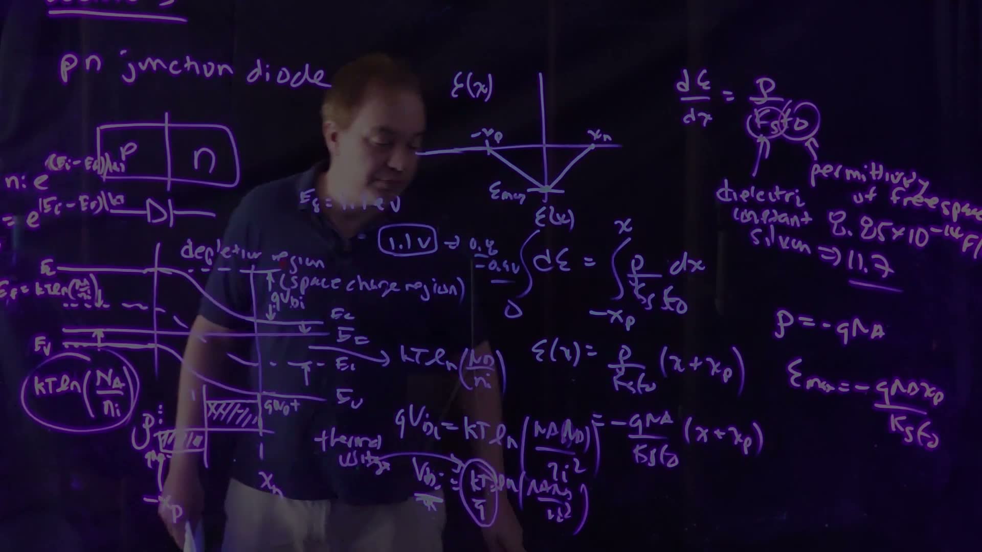
Lecture 2 ended with the junction’s band diagram in equilibrium: one flat Fermi level, p-type bands on the left, n-type on the right, and a region of band bending in between. The bending region is the depletion region, also called the space-charge region. It holds almost no mobile carriers but does hold fixed charge:

on the p side, ionized acceptors: $\rho = -qN_A$ for $-x_p < x < 0$ ;
on the n side, ionized donors: $\rho = +qN_D$ for $0 < x < x_n$ .

Here $x = 0$ is the metallurgical junction, where the doping switches from p to n. $x_p$ and $x_n$ are how far the depletion region reaches into each side. Treating the charge as these two clean rectangles is the depletion approximation.

Lightboard: pn junction diode with its band diagram, the charge density rectangles, the triangular electric field with E_max at the junction, Gauss's law integrated from −x_p, and the built-in voltage formula. — Lecture03 @ 10:22The junction board: band diagram (left), charge and field (centre), Gauss's law and the built-in voltage (right and bottom).

The field: integrate the charge once

Start in the neutral p region, where the field is zero, and integrate Gauss’s law to a point $x$ inside the p-side depletion region:

Field on the p side (board, 2:12–4:50)

Gauss’s law board: $\dfrac{d\mathcal{E}}{dx} = \dfrac{\rho}{\kappa_s\varepsilon_0}$ .
Integrate from $-x_p$ , where $\mathcal{E} = 0$ : $\displaystyle\int_0^{\mathcal{E}(x)} d\mathcal{E} = \int_{-x_p}^{x} \frac{\rho}{\kappa_s\varepsilon_0}\,dx$ .
The charge is constant there, so $\mathcal{E}(x) = \dfrac{\rho}{\kappa_s\varepsilon_0}(x + x_p)$ .
Substitute $\rho = -qN_A$ : $\mathcal{E}(x) = -\dfrac{qN_A}{\kappa_s\varepsilon_0}(x + x_p)$ . It is a straight line, falling from zero at $-x_p$ .
At the junction ( $x = 0$ ) the field is largest in size: $\mathcal{E}_{max} = -\dfrac{qN_A x_p}{\kappa_s\varepsilon_0}$ .

Continue into the n side. Now the positive donor charge makes the field climb back, linearly, and it reaches zero exactly at $x_n$ . It must: the field is zero in the neutral n region too, which is only possible if the total charge is zero. So the field is a triangle, with its tip at the junction.

The field is negative everywhere in the depletion region: it points from the positive (n) side to the negative (p) side, that is, toward $-x$ .

The potential: integrate again

Integrating a linear field gives a quadratic potential. That is exactly the S-shaped curve of the band bending: $E_C$ , $E_i$ and $E_V$ all follow $-q\psi(x)$ . The lecturer puts it as “I integrate a constant, I get a linear; I integrate a linear, I get a quadratic” (5:25).

Check yourself Why must the two shaded areas of the charge-density plot be equal?

Because the field is zero outside the depletion region on both sides. Integrating Gauss’s law across the whole junction, the change in field equals the total charge (per area) divided by $\kappa_s\varepsilon_0$ . A zero change requires zero total charge: $qN_Ax_p = qN_Dx_n$ .

Common mistakes.

Putting the peak field anywhere but the metallurgical junction. The field keeps growing in size as long as you integrate charge of one sign, and the sign flips at $x = 0$ .
Thinking the depletion regions on the two sides have equal widths. They have equal charge; the lightly doped side depletes farther.

2. The built-in voltage

The idea. The potential step across the junction, $V_{bi}$ , is fixed by how far each side’s Fermi level sits from mid-gap. You can read it straight off the band diagram.

In equilibrium the Fermi level is flat, so the band bending must make up the difference between the two sides’ $E_i$ positions.

Built-in voltage from the band diagram (board, 6:30–8:30)

On the p side, $p = N_A = n_i e^{(E_i - E_F)/kT}$ , so $E_i - E_F = kT\ln(N_A/n_i)$ . This is the circled spacing on the board.
On the n side, $n = N_D = n_i e^{(E_F - E_i)/kT}$ , so $E_F - E_i = kT\ln(N_D/n_i)$ .
The total bending is the sum: $qV_{bi} = kT\ln\dfrac{N_A}{n_i} + kT\ln\dfrac{N_D}{n_i} = kT\ln\dfrac{N_AN_D}{n_i^2}$ .
Divide by $q$ board: $V_{bi} = \dfrac{kT}{q}\ln\dfrac{N_AN_D}{n_i^2}$ .

How large can $V_{bi}$ be? The lecturer asks this himself (8:43). The best you can do is push $E_F$ all the way to $E_V$ on the p side and to $E_C$ on the n side, with very heavy doping. Each spacing is then about half the band gap, so $V_{bi}$ can never exceed about $E_g/q = 1.1\,\mathrm{V}$ . For ordinary doping it is about 0.8–0.9 V. The band gap fixes this number, and it can’t be scaled down. The lecturer flags that this will matter later, when supply voltages shrink with scaling (10:10–10:40).

Worked example. added $N_A = 10^{17}\,\mathrm{cm^{-3}}$ , $N_D = 10^{16}\,\mathrm{cm^{-3}}$ .

$N_AN_D/n_i^2 = 10^{17}\cdot10^{16}/10^{20} = 10^{13}$ .
$\ln(10^{13}) = 13 \times 2.303 = 29.93$ .
$V_{bi} = 0.02585 \times 29.93 = 0.774\,\mathrm{V}$ . The rule of thumb gives the same: 13 decades × 60 mV ≈ 0.78 V.

Check yourself Both sides are doped 10× more heavily. By how much does V_bi rise?

$N_AN_D$ grows by 100, so $V_{bi}$ rises by $\frac{kT}{q}\ln 100 \approx 0.12\,\mathrm{V}$ , about 60 mV for each factor of 10.

3. The depletion width

The idea. Two facts fix the width: the charges on the two sides balance, and the area of the field triangle equals the voltage across the junction.

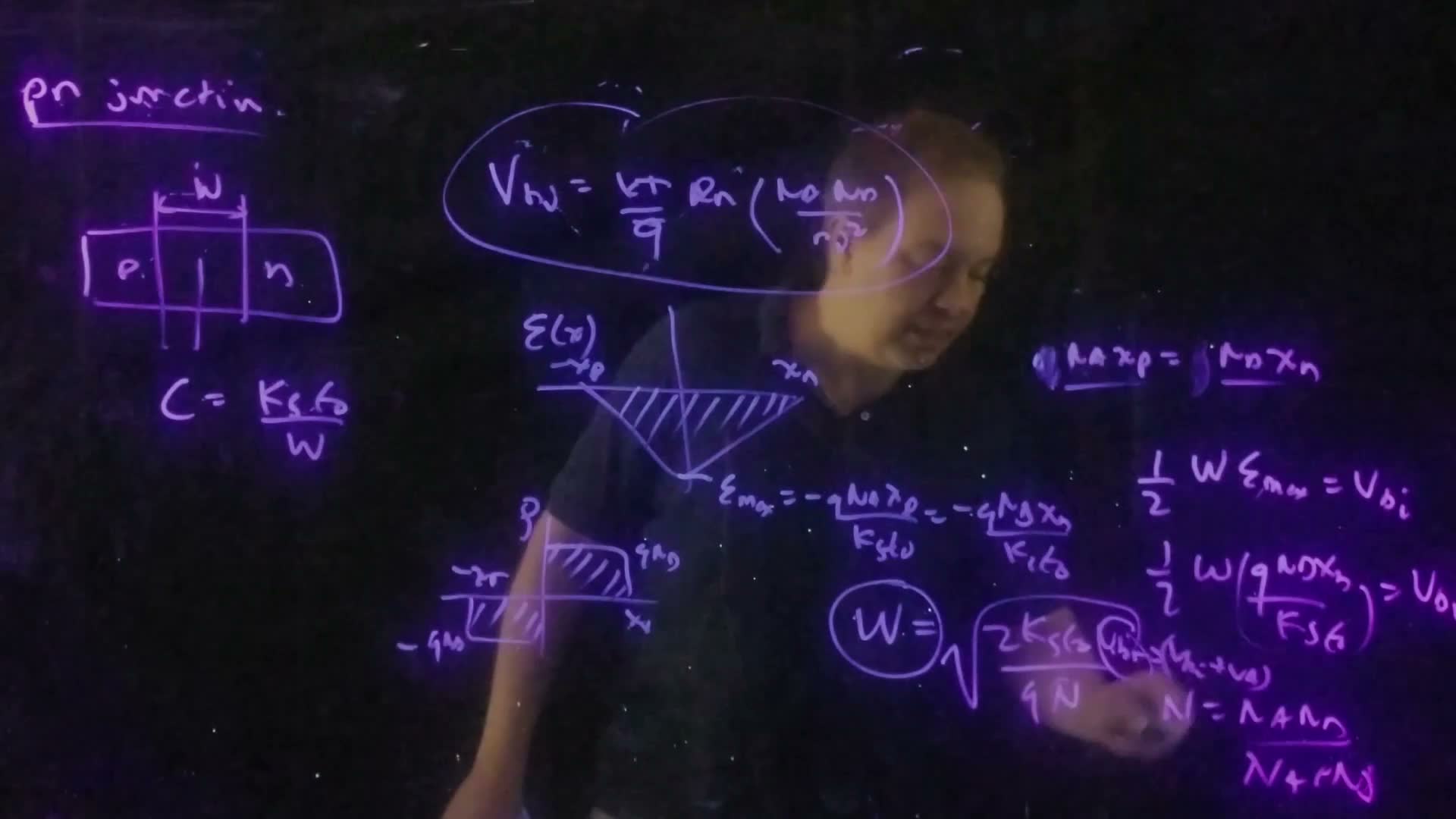
Lightboard: V_bi formula circled, C = κsε0/W, field triangle with E_max expressions, charge density rectangles, the conditions qN_A x_p = qN_D x_n and ½ W E_max = V_bi, and the boxed depletion-width formula with N = N_A N_D / (N_A + N_D). — Lecture03 @ 20:00The depletion-width derivation, written after a camera problem wiped the earlier board.

Depletion width (board, 17:28–19:30)

Charge balance: $qN_Ax_p = qN_Dx_n$ . So the peak field can be written either way: $\mathcal{E}_{max} = -\dfrac{qN_Ax_p}{\kappa_s\varepsilon_0} = -\dfrac{qN_Dx_n}{\kappa_s\varepsilon_0}$ .
Triangle area = voltage. The potential step is the area under the field, $\tfrac12 \times \text{base} \times \text{height}$ : $\tfrac12 W|\mathcal{E}_{max}| = V_{bi}$ , with $W = x_n + x_p$ .
Use charge balance to write each side’s width as a share of $W$ added: $x_n = W\dfrac{N_A}{N_A + N_D}$ and $x_p = W\dfrac{N_D}{N_A + N_D}$ .
Substitute into the area: $\tfrac12 W \cdot \dfrac{qN_D}{\kappa_s\varepsilon_0}\cdot W\dfrac{N_A}{N_A+N_D} = V_{bi}$ , that is, $\dfrac{qNW^2}{2\kappa_s\varepsilon_0} = V_{bi}$ with $N = \dfrac{N_AN_D}{N_A+N_D}$ .
Solve for $W$ : $W = \sqrt{\dfrac{2\kappa_s\varepsilon_0 V_{bi}}{qN}}$ .

Explore the junction below. Change the doping on each side and the reverse bias, and watch all four pictures update together.

What to notice.

Make one side much more heavily doped (say $N_A = 10^{19}$ , $N_D = 10^{16}$ ). Nearly all the depletion width moves into the light side, and $N \approx N_D$ . This is a one-sided junction, which is what a transistor’s $n^+$ source or drain in a p body looks like.
The charge rectangles always have equal areas, and the field triangle always closes at zero.
Raising $V_R$ widens the depletion region, deepens the field triangle and raises the band step. The depletion width grows only as $\sqrt{V_{bi} + V_R}$ .

Worked example. added Same junction, $N_A = 10^{17}$ , $N_D = 10^{16}\,\mathrm{cm^{-3}}$ , no bias.

$N = 10^{33}/(1.1\times10^{17}) = 9.09\times10^{15}\,\mathrm{cm^{-3}}$ , a bit below the lighter doping.
$W = \sqrt{\dfrac{2(1.036\times10^{-12})(0.774)}{(1.602\times10^{-19})(9.09\times10^{15})}} = 3.32\times10^{-5}\,\mathrm{cm} = 0.332\,\mu\mathrm{m}$ .
Split: $x_n = W \cdot 10/11 = 0.302\,\mu\mathrm{m}$ and $x_p = W/11 = 0.030\,\mu\mathrm{m}$ . Ten times the doping, one tenth the width.
Peak field: $|\mathcal{E}_{max}| = 2V_{bi}/W = 2(0.774)/(3.32\times10^{-5}) = 4.66\times10^4\,\mathrm{V/cm}$ , about 47 kV/cm.

Check yourself N_A = 4 N_D. What fraction of W lies on the n side?

$x_n/W = N_A/(N_A+N_D) = 4/5$ . The n side is the lighter one, so it holds 80% of the width.

4. Reverse bias

The idea. A reverse bias adds to the built-in voltage. The barrier gets taller, the depletion region wider and the peak field stronger, while almost no current flows.

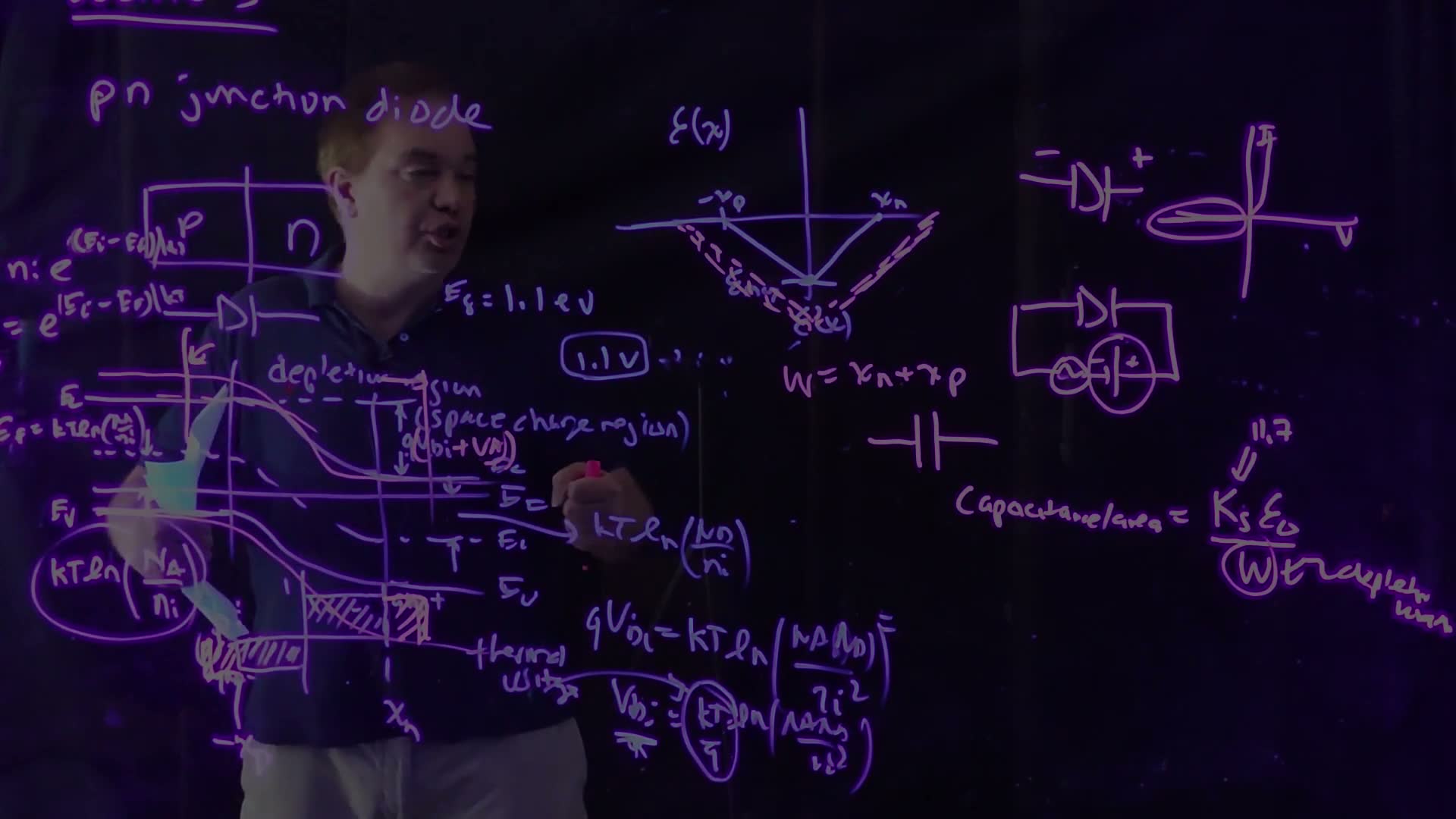
Reverse bias means making the n side positive relative to the p side (11:07). The applied voltage then adds to $V_{bi}$ , so the total voltage across the depletion region becomes $V_{bi} + V_R$ (12:36):

the barrier for electrons grows from $qV_{bi}$ to $q(V_{bi} + V_R)$ ;
to hold more voltage, the junction must expose more fixed charge, so the depletion region widens;
more charge means a deeper field triangle, so the peak field grows.

Only a tiny reverse leakage current flows. This is the left half of the diode’s I–V curve on the board at 15:40.

Lightboard: the junction band diagram relabelled q(V_bi + V_A), a larger dashed field triangle, W = x_n + x_p, the diode I–V curve, a diode with a DC source and a small AC source, a capacitor symbol, and capacitance per area = κsε0/W with 11.7 marked. — Lecture03 @ 15:40Reverse bias widens the field triangle (dashed). Capacitance per area κsε0/W is at the right.

In a MOS transistor, the source–body and drain–body junctions are always zero- or reverse-biased (11:07). That is why the lecture spends time on this case.

Check yourself Doubling (V_bi + V_R) multiplies W by what factor? And the peak field?

$W \propto \sqrt{V_{bi}+V_R}$ , so $W$ grows by $\sqrt2 \approx 1.41$ . The peak field is $2(V_{bi}+V_R)/W$ , so it also grows by $2/\sqrt2 = \sqrt2$ .

5. The junction is a capacitor

The idea. A small extra voltage on a reverse-biased junction moves a small amount of charge at the depletion edges. That is a capacitor whose plate spacing is the depletion width.

Put a small AC signal on top of the DC reverse bias (13:44). Each wiggle of voltage pushes the edges $-x_p$ and $x_n$ in and out a little. That uncovers or covers a sliver of ion charge on each side, equal and opposite, like charge on two plates. To a circuit, the junction looks like a parallel-plate capacitor with silicon as the dielectric and $W$ as the spacing.

Why exactly $\kappa_s\varepsilon_0/W$ ? added The charge on one side is $Q = qNW$ , and $W^2 = 2\kappa_s\varepsilon_0(V_{bi}+V_R)/(qN)$ . Differentiate: $2W\,dW = (2\kappa_s\varepsilon_0/qN)\,dV_R$ , so $dQ/dV_R = qN\,dW/dV_R = \kappa_s\varepsilon_0/W$ . The small-signal capacitance $dQ/dV$ comes out exactly like a parallel plate.

The key consequence. As reverse bias grows, $W$ grows, so $C_j$ falls (15:24). A reverse-biased junction is a capacitor whose value depends on its voltage. This matters later, because these junction capacitances load every logic gate’s output.

Worked example. added The same junction, at $V_R = 0$ and at $V_R = 2\,\mathrm{V}$ .

$V_R = 0$ : $C_j = 1.036\times10^{-12}/3.32\times10^{-5} = 3.12\times10^{-8}\,\mathrm{F/cm^2} = 0.31\,\mathrm{fF/\mu m^2}$ .
$V_R = 2\,\mathrm{V}$ : $V_{bi} + V_R = 2.774\,\mathrm{V}$ , so $W$ grows by $\sqrt{2.774/0.774} = 1.893$ to $0.628\,\mu\mathrm{m}$ .
$C_j = 1.036\times10^{-12}/6.28\times10^{-5} = 1.65\times10^{-8}\,\mathrm{F/cm^2}$ , down to 53% of its zero-bias value.
For a $100\,\mu\mathrm{m^2}$ junction: 31 fF at 0 V, 16 fF at 2 V.

Common mistakes.

Expecting capacitance to rise with voltage because the stored charge rises. The charge does rise, but as $\sqrt{V}$ , whose slope falls. Capacitance is the slope.
Using $\kappa_{ox}$ (3.9) here. The dielectric of a junction capacitor is silicon (11.7).

Check yourself What reverse bias halves C_j relative to zero bias?

$C_j \propto 1/\sqrt{V_{bi}+V_R}$ . Halving it needs $V_{bi}+V_R = 4V_{bi}$ , so $V_R = 3V_{bi}$ , about 2.3 V for this junction.

6. The MOS transistor: structure

The idea. A MOS transistor is a p-type body with two $n^+$ islands, the source and drain, and a gate sitting on a thin insulator over the gap between them.

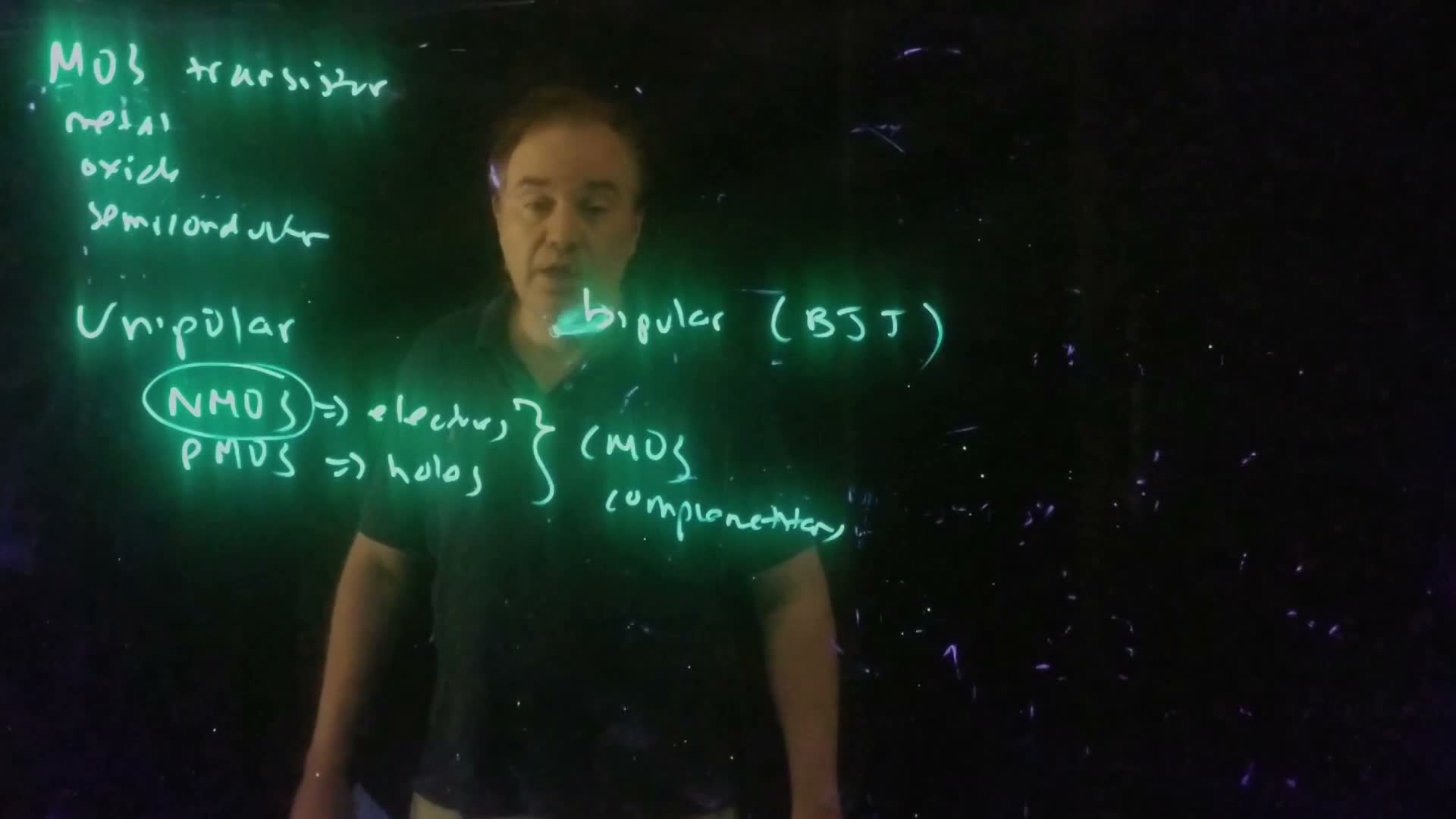
MOS stands for metal–oxide–semiconductor, the three layers stacked under the gate (20:58).

Lightboard: MOS transistor = metal, oxide, semiconductor; unipolar versus bipolar (BJT); NMOS ⇒ electrons, PMOS ⇒ holes; CMOS = complementary. — Lecture03 @ 22:32Unipolar device; NMOS uses electrons, PMOS uses holes; CMOS has both.

Unipolar, NMOS and PMOS

A bipolar device, such as the bipolar junction transistor (BJT), can only be understood by following both electrons and holes.
A MOS transistor is unipolar: its operation depends on one carrier type (21:07–21:42).
- NMOS conducts with electrons.
- PMOS conducts with holes.
A technology that offers both is CMOS, complementary MOS (21:59).

A bit of history from the lecture: early MOS technologies could make only NMOS. Circuit styles from that era, pseudo-NMOS and dynamic logic, still appear later in the course. Mead and Conway’s textbook (1980), the first VLSI text, was NMOS-only (22:27). The lecture analyses the NMOS device; PMOS works the same way with every sign flipped, which you practise in the problem set (22:58).

Cross-section and terminals

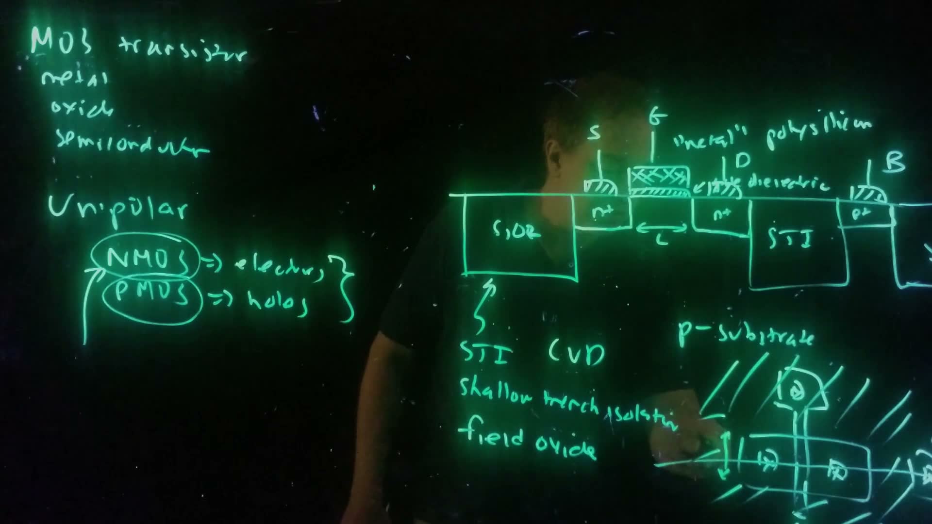
Lightboard: NMOS cross-section with SiO2 shallow trench isolation, n+ source and drain, thin gate dielectric, polysilicon 'metal' gate, p+ body contact, terminals S, G, D, B, channel length L, p-substrate; notes STI, CVD, shallow trench isolation, field oxide; top view with source, gate, drain and width W at the bottom right. — Lecture03 @ 28:34Side view of an NMOS transistor (top right) and top view (bottom right).

Reading the cross-section from left to right (23:23–26:13):

Shallow trench isolation (STI): trenches etched into the silicon and filled with deposited oxide (CVD, chemical vapour deposition). It isolates neighbouring devices. Older processes grew a thick field oxide instead. That doesn’t scale well, because the oxide grows sideways into “bird’s beaks”.
Source and drain: $n^+$ regions, ion-implanted and diffused into the p-type substrate.
Body contact: a $p^+$ region tying the substrate to a terminal. It is often shared with other devices.
Gate dielectric: a thin insulator, traditionally SiO₂. Newer processes use high-κ metal oxides, but still rely on the good interface between SiO₂ and silicon.
Gate: a conductor. Traditionally it is polysilicon, heavily doped polycrystalline silicon that acts as a (resistive) metal and has a convenient work function (Section 9). Modern processes use real metal gates.

So a MOS transistor has four terminals: source, gate, drain and body (S, G, D, B). The body terminal matters, and Chapter 5 returns to it.

Source and drain are interchangeable. The device is symmetric, so which end is the source depends only on how it is biased, and the roles can swap while a circuit runs. A pass transistor is the example (26:13–27:16). A BJT is different: its emitter and collector are built differently, and running it backwards gives a poor transistor.

Length and width

From the top view (27:38–28:58):

Channel length $L$ : the gate’s extent from source to drain. It is usually the smallest dimension the lithography can draw, and digital circuits nearly always use the minimum $L$ . That minimum is what names the technology node (Chapter 1).
Width $W$ : the gate’s extent across the channel. Width is the designer’s main knob, because the transistor’s current drive scales with it. Most of this course is about choosing widths for the load a transistor drives.

Don’t confuse this $W$ (transistor width) with the junction depletion width $W$ above. The board uses the same letter for both.

Check yourself A transistor's source and drain are swapped in the layout. Does the circuit behave differently?

No. The planar MOS transistor is symmetric. Whichever $n^+$ region is at the lower potential acts as the source (for NMOS). Only biasing decides.

7. The MOS capacitor: depletion, then inversion

The idea. A positive gate voltage first pushes holes away from the surface, leaving negative acceptor ions (depletion). Push harder and the bands bend so far that electrons collect at the surface: an n-type layer forms in p-type silicon (inversion).

The setup

Ground the source, drain and body, apply $V_{GB}$ between gate and body, and look at a vertical slice through the gate (28:58–29:48). That slice is a MOS capacitor: metal, oxide and p-type silicon.

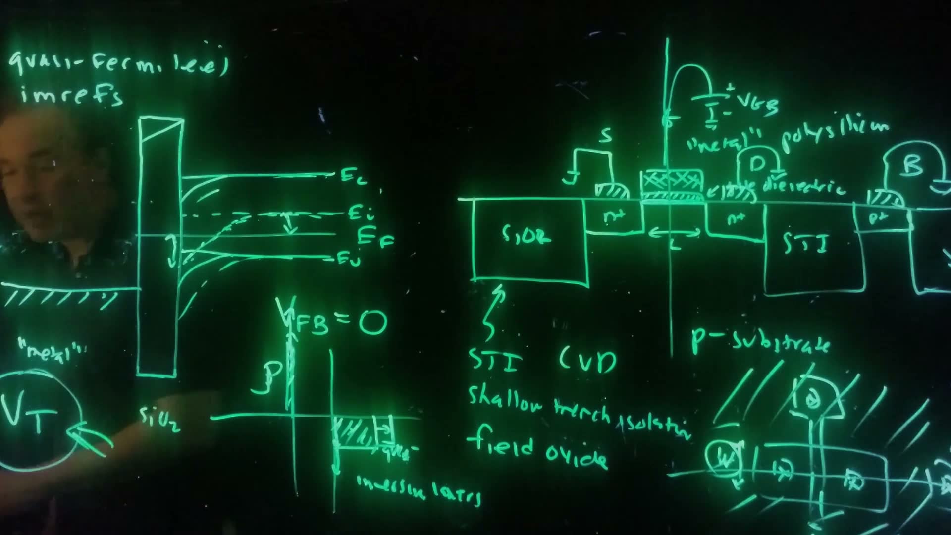
Lightboard: MOS band diagram with the metal (hatched) at left, the tall SiO2 box, and p-silicon bands E_C, E_i, E_F, E_V bending down at the surface; labels quasi-Fermi level and imrefs; V_FB = 0; charge plot with a positive sheet at the gate, depletion charge and an inversion layer; V_T circled; the transistor with V_GB applied, S, D and B grounded. — Lecture03 @ 36:11The MOS band diagram under positive gate bias (left), its charge (centre bottom), and the bias setup (right).

Band diagram at zero bias (29:48–31:39):

the metal: a Fermi level with filled states below it (the hatched line);
the oxide: drawn as a very wide-gap semiconductor (the gap of SiO₂ is about 8 eV);
the p-type silicon: Fermi level in the lower half of the gap.

The lecture first assumes that with $V_{GB} = 0$ all bands are flat and there is no charge anywhere. This is the flat-band condition. In general, flat bands need a particular gate voltage, the flat-band voltage $V_{FB}$ . For now, $V_{FB} = 0$ ; Section 9 removes this assumption.

Positive gate voltage

Applying $V_{GB}$ takes the structure out of equilibrium, so the Fermi levels on the two sides separate by $qV_{GB}$ . The lecturer calls them quasi-Fermi levels. He mentions the cute name “imrefs” (Fermi spelled backwards) only to say he won’t use it (31:39–32:48). A positive $V_{GB}$ pulls the metal’s level down by $qV_{GB}$ , and the silicon bands bend down toward the surface.

Now follow the charge as $V_{GB}$ rises:

Depletion (32:50). Downward bending pushes holes away from the surface, uncovering acceptor ions: a depletion region of charge $-qN_A$ , just as on the p side of a junction. An equal positive charge appears on the gate, as a thin sheet against the oxide. The two balance, so the field is zero deep in the silicon.
The depletion region grows as $V_{GB}$ rises and the bending increases.
Inversion (34:15). Eventually the surface $E_i$ drops below $E_F$ . Electrons now outnumber holes there: the surface has inverted to n-type. The standard criterion is the point where $E_i$ at the surface is as far below $E_F$ as it is above $E_F$ in the bulk. This is strong inversion, and the gate voltage that reaches it is the threshold voltage $V_T$ (34:45–35:27).
Above threshold. The depletion region stops growing. Its maximum depth is $W_{dmax}$ . Any further gate charge is balanced by electrons in the thin inversion layer at the surface (34:25).

Why it matters. The inversion layer is a sheet of electrons connecting the $n^+$ source to the $n^+$ drain. Below $V_T$ there is no such path, and the transistor is off. Above $V_T$ the path exists, and the transistor is on. This is how the MOS transistor works as a switch (35:27–35:53).

Explore the MOS capacitor below. Press Play sweep to raise $V_{GB}$ from −1 V to 3 V and watch the inversion layer form.

gate-to-body voltage V_GB0.00 V

flat band: V_GB = V_FB, so the bands are flat and there is no charge anywhere.

V_T (lecture model): 1.074 V
ψ_s (band bending): 0.000 V; 2φ_F = 0.833 V
voltage across oxide: 0.000 V
W_d (W_dmax): 0.0 (103.8) nm
depletion charge: 0 C/cm²
electron (inversion) charge: 0 C/cm²

What to notice.

Accumulation (below $V_{FB}$ ): the bands bend up and holes pile up at the surface. The lecture doesn’t discuss this case, but the widget shows it for completeness.
Depletion: the shaded depletion region deepens and the band bending $\psi_s$ rises quickly with $V_{GB}$ .
Inversion: once $\psi_s$ nears $2\phi_F$ , it nearly stops rising. Extra gate voltage now goes almost entirely into electrons, and $|Q_{inv}|$ grows along the straight line $C_{ox}(V_{GB} - V_T)$ .
The full model (solid curve) turns on smoothly, not abruptly at $V_T$ . $V_T$ is a well-defined criterion on a smooth curve. Lecture 4 uses the straight-line part.
In the full model the depletion depth still creeps past $W_{dmax}$ above threshold, by about 10% at 2 V above threshold, because $\psi_s$ rises a few $kT/q$ . The lecture’s “it stops growing” is the standard approximation.

Check yourself Above threshold, why doesn't the depletion region keep growing?

At strong inversion the surface electron population grows exponentially with any extra band bending. A tiny increase in $\psi_s$ supplies all the extra negative charge as electrons. So $\psi_s$ , and with it the depletion depth, stays almost fixed at its threshold value, $W_{dmax}$ .

8. The threshold voltage

The idea. At threshold, the gate voltage is split between two drops: the band bending in the silicon, $2\phi_F$ , and the voltage across the oxide needed to hold the depletion charge.

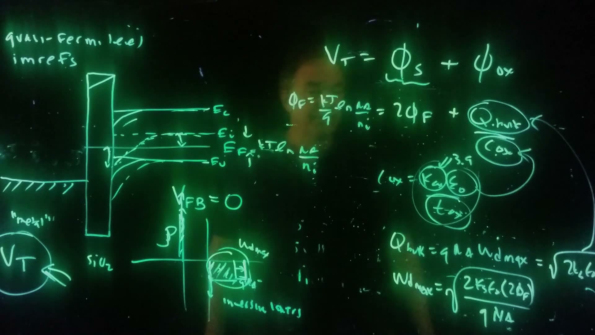
Lightboard: V_T = φ_s + φ_ox; φ_F = (kT/q) ln(N_A/n_i); φ_s = 2φ_F; φ_ox = Q_bulk / C_ox; C_ox = κ_ox ε0 / t_ox with 3.9; Q_bulk = q N_A W_dmax; W_dmax = sqrt(2 κs ε0 (2φ_F) / (q N_A)); the MOS band diagram with kT ln(N_A/n_i) marked. — Lecture03 @ 41:08The threshold derivation. The right edge of the Q_bulk line runs off the frame; the transcript completes it.

Threshold voltage (board, 37:06–41:03)

Split the gate voltage board: $V_T = \phi_s + \phi_{ox}$ , the voltage dropped in the semiconductor plus the voltage across the oxide (with $V_{FB} = 0$ ).
The bulk spacing $E_i - E_F = kT\ln(N_A/n_i)$ , written as a voltage board: $\phi_F = \dfrac{kT}{q}\ln\dfrac{N_A}{n_i}$ .
At strong inversion, the surface $E_i$ must be pulled from $q\phi_F$ above $E_F$ to $q\phi_F$ below it, a total of $2q\phi_F$ . So $\phi_s = 2\phi_F$ .
The oxide is a capacitor holding the depletion charge: $\phi_{ox} = Q_{bulk}/C_{ox}$ , with $C_{ox} = \kappa_{ox}\varepsilon_0/t_{ox}$ per area ( $\kappa_{ox} = 3.9$ ).
The depletion charge is $Q_{bulk} = qN_AW_{dmax}$ .
$W_{dmax}$ follows exactly as for a one-sided junction, with $2\phi_F$ across the depletion region: $W_{dmax} = \sqrt{\dfrac{2\kappa_s\varepsilon_0(2\phi_F)}{qN_A}}$ .
Combine 5 and 6: $Q_{bulk} = \sqrt{2\kappa_s\varepsilon_0\,(2\phi_F)\,qN_A}$ , as spoken at 40:50.

Where $2\phi_F$ comes from, in carrier terms. added The Fall 2026 class added this. Bending the bands down by $\psi_s$ multiplies the surface electron concentration by $e^{q\psi_s/kT}$ : $n_s = (n_i^2/N_A)\,e^{q\psi_s/kT}$ . At $\psi_s = 2\phi_F$ , $e^{q\psi_s/kT} = (N_A/n_i)^2$ , so $n_s = N_A$ . Strong inversion means the surface has as many electrons as the bulk had holes.

Worked example. added $N_A = 10^{17}\,\mathrm{cm^{-3}}$ , $t_{ox} = 5\,\mathrm{nm}$ , $V_{FB} = 0$ .

$\phi_F = 0.02585\ln(10^{17}/10^{10}) = 0.02585 \times 16.12 = 0.417\,\mathrm{V}$ , so $2\phi_F = 0.833\,\mathrm{V}$ .
$C_{ox} = 3.9 \times 8.854\times10^{-14}/(5\times10^{-7}) = 6.91\times10^{-7}\,\mathrm{F/cm^2}$ .
$W_{dmax} = \sqrt{\dfrac{2(1.036\times10^{-12})(0.833)}{1.602\times10^{-19}\times10^{17}}} = 1.04\times10^{-5}\,\mathrm{cm} = 0.104\,\mu\mathrm{m}$ .
$Q_{bulk} = qN_AW_{dmax} = 1.602\times10^{-19}\times10^{17}\times1.04\times10^{-5} = 1.66\times10^{-7}\,\mathrm{C/cm^2}$ .
$\phi_{ox} = Q_{bulk}/C_{ox} = 1.66\times10^{-7}/6.91\times10^{-7} = 0.241\,\mathrm{V}$ .
$V_T = 0.833 + 0.241 = 1.07\,\mathrm{V}$ . Most of it is band bending; the oxide takes about a fifth.

Common mistakes.

Using $\phi_F$ instead of $2\phi_F$ . At $\psi_s = \phi_F$ the surface is merely intrinsic.
Multiplying by $C_{ox}$ instead of dividing. The spoken words at 39:44 say “Q bulk times C ox”, but the board is right: a voltage is charge divided by capacitance.
Using $\kappa_s$ in $C_{ox}$ . The oxide’s permittivity is $3.9\,\varepsilon_0$ .

Check yourself The oxide is made twice as thick. Which terms of V_T change?

Only the oxide term. $C_{ox}$ halves, so $Q_{bulk}/C_{ox}$ doubles (0.241 → 0.482 V in the example). $\phi_F$ and $W_{dmax}$ depend only on the body doping.

9. Flat-band voltage and the work function

The idea. The metal and the semiconductor generally hold their electrons at different depths below the vacuum level. Joining them bends the bands even at zero bias, and the gate voltage that undoes that bending is $V_{FB}$ .

Lightboard: 'work function difference' with a vacuum level, the metal work function from E_F to vacuum, a semiconductor band diagram with its own work function, V_FB ≠ 0; V_T = φ_s + φ_ox + V_FB; threshold set by (1) doping and (2) work function engineering, with notes 'random dopant fluctuation' and N_A circled in blue. — Lecture03 @ 49:22Work function, V_FB ≠ 0, and the two ways to set V_T. The expression after 'V_FB =' at the top right runs off the frame.

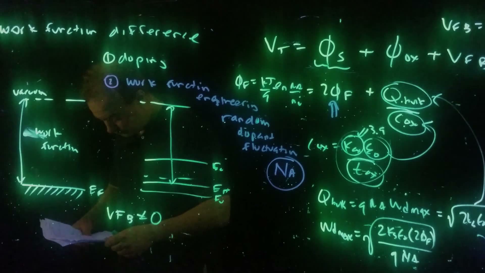
The lecturer motivates this with the photoelectric effect, the work Einstein actually won his Nobel Prize for (42:20–43:24). Shine light of high enough energy on a metal and an electron is kicked out of the metal entirely, from the Fermi level up to the vacuum level. The energy needed is the work function:

\text{work function} = E_{vacuum} - E_F .

A semiconductor has a work function too. Because doping moves $E_F$ within the gap, a semiconductor’s work function depends on its doping (43:36).

If the gate and the silicon have different work functions, their Fermi levels can only line up in equilibrium if the bands bend. So even at $V_{GB} = 0$ the bands are not flat, and a gate voltage $V_{FB}$ is needed to flatten them (44:13). Threshold is then reached by applying $V_{FB}$ first and the inversion voltage on top:

V_T = \phi_s + \phi_{ox} + V_{FB} .

The formula for $V_{FB}$ added. The board’s " $V_{FB} =$ " runs off the frame. The standard result, also the Fall 2026 board’s, is the work-function difference in volts, $V_{FB} = \phi_m - \phi_s$ (metal minus semiconductor), for an ideal oxide with no trapped charge. Note the name clash: this $\phi_s$ is the semiconductor’s work function, not the surface potential.

Worked example. added The same device with $V_{FB} = -0.30\,\mathrm{V}$ : $V_T = -0.30 + 0.833 + 0.241 = 0.774\,\mathrm{V}$ . The work-function difference shifts $V_T$ one-for-one.

10. What sets the threshold in practice

The lecture closes with two levers (44:41–49:36).

(1) Doping. $N_A$ enters $V_T$ strongly through $Q_{bulk} \propto \sqrt{N_A}$ , and weakly (logarithmically) through $\phi_F$ . Real devices engineer not just the doping level but the doping profile: non-uniform doping under the gate controls short-channel effects (Lecture 4) as well as $V_T$ (45:19–46:11). The uniform- $N_A$ formula is a model, not the real device.

The problem with doping at small sizes: random dopant fluctuations (46:24–48:12). In a tiny transistor, the number of dopant atoms under the gate becomes countable, say about 30. One device gets 28, the next 32, and their thresholds differ noticeably. The dopants’ positions also vary. This threshold variability is especially harmful in SRAM cells, which depend on the strength ratios of their transistors. Mismatched thresholds can leave random bits in a cache that simply don’t work.

(2) Work-function engineering (48:24–49:05). One fix is to remove the doping. Fully depleted device structures use essentially undoped channels and set $V_T$ by choosing the gate metal’s work function, that is, through $V_{FB}$ . No dopants means no random dopant fluctuations.

Check yourself Why does a 'countable' number of dopants cause threshold variation, when the average doping is exactly as designed?

Each device samples a random number of dopants around the average. With about 30 dopants, the statistical spread is about ±√30 ≈ ±5.5, roughly 18% (an added Poisson-counting estimate, not from the board). The depletion charge, and with it $V_T$ , varies device to device by a comparable fraction of its doping-dependent part.

Formulas to remember

Formula	Meaning
$V_{bi} = \dfrac{kT}{q}\ln\dfrac{N_AN_D}{n_i^2}$	built-in voltage, at most about $E_g/q$
$qN_Ax_p = qN_Dx_n$	charge balance
$\mathcal{E}_{max} = -\dfrac{qN_Ax_p}{\kappa_s\varepsilon_0}$ , $\tfrac12 W\lvert\mathcal{E}_{max}\rvert = V_{bi}+V_R$	peak field; triangle area
$W = \sqrt{\dfrac{2\kappa_s\varepsilon_0(V_{bi}+V_R)}{qN}}$ , $N = \dfrac{N_AN_D}{N_A+N_D}$	depletion width
$C_j = \kappa_s\varepsilon_0/W$	junction capacitance per area; falls with reverse bias
$\phi_F = \dfrac{kT}{q}\ln\dfrac{N_A}{n_i}$ , $\phi_s = 2\phi_F$ at threshold	band bending to invert
$C_{ox} = \kappa_{ox}\varepsilon_0/t_{ox}$	oxide capacitance per area
$W_{dmax} = \sqrt{\dfrac{2\kappa_s\varepsilon_0(2\phi_F)}{qN_A}}$ , $Q_{bulk} = qN_AW_{dmax}$	depletion depth and charge at threshold
$V_T = V_{FB} + 2\phi_F + Q_{bulk}/C_{ox}$	threshold voltage

The lecture’s boards

Lecture03 board at 10:22: pn junction: charge, field, Vbi — Lecture03 @ 10:22 pn junction: charge, field, V_bi

Lecture03 board at 15:40: reverse bias and capacitance per area — Lecture03 @ 15:40 reverse bias and capacitance per area

Lecture03 board at 20:00: depletion width W — Lecture03 @ 20:00 depletion width W

Lecture03 board at 22:32: MOS: unipolar, NMOS/PMOS, CMOS — Lecture03 @ 22:32 MOS: unipolar, NMOS/PMOS, CMOS

Lecture03 board at 28:34: NMOS cross-section and top view — Lecture03 @ 28:34 NMOS cross-section and top view

Lecture03 board at 36:11: MOS band bending and inversion — Lecture03 @ 36:11 MOS band bending and inversion

Lecture03 board at 41:08: threshold voltage derivation — Lecture03 @ 41:08 threshold voltage derivation

Lecture03 board at 49:22: work function, VFB, doping vs work-function engineering — Lecture03 @ 49:22 work function, V_FB, doping vs work-function engineering