1. The big picture

Lecture 1 has no equations. It sets the stage: why transistors keep getting smaller and what that bought, how engineers manage chips with tens of billions of transistors, and why the course builds on silicon CMOS. It ends with the device-physics road map that Lectures 2–5 follow. Read this chapter for the vocabulary and the reasons; every number in it comes back later with a formula behind it.

After this chapter you can:

1. say what Moore’s law and Dennard scaling each promised, and which of the two has stopped;
2. explain what a technology node names, and generate the node sequence from 1 µm with the factor $1/\sqrt2$1/2​;
3. list the levels of abstraction from devices to the system, and the CAD tool that moves or checks between each pair;
4. explain why digital circuits tolerate noise and variability, and why some functions still have to be analog;
5. give the lecture’s reasons for silicon over gallium arsenide, and for CMOS over bipolar logic.

Boxes and statements marked board were written in the lecture. Parts marked added are explanations or examples this guide adds.

Before you start

This chapter needs only two small tools.

• Repeated scaling factors. Multiplying a length by $1/\sqrt2 \approx 0.707$ multiplies an area by $(1/\sqrt2)^2 = 1/2$1/2. Two such steps halve the length.
• Frequency and period. A clock with cycle time $T$ runs at $f = 1/T$1/T. For example, $1/(1\,\mathrm{ns}) = 1\,\mathrm{GHz}$1GHz.

1. What the course covers

The idea. E4321 builds digital circuits up from the transistor. The device physics comes first because every later sizing and delay rule rests on it.

The lecture’s outline of the term (6:58–9:15):

• Before the midterm: semiconductor device physics and combinational logic design, including standard-cell logic and its sizing, dynamic logic, and the start of sequential design (latches and clocking).
• After the midterm: what the design project needs. These are the building blocks of a microprocessor (datapath elements, control logic, memories) and the problems of integrating them.
• At the end, if time allows: testability, packaging and I/O.

The textbook is Weste and Harris, CMOS VLSI Design, fourth edition only (1:38). It is recommended, not required. The lecturer doesn’t lecture out of the book: it covers similar material in a different way, so use it as a second explanation.

Books on reserve (4:50–6:58), for when you want more:

Book	What it’s good for
Rabaey, Digital Integrated Circuits	the course’s earlier textbook
Glasser and Dobberpuhl, The Design and Analysis of VLSI Circuits	older (“very dated”) but still excellent on several topics
Taur and Ning, Fundamentals of Modern VLSI Devices	device physics; the early device lectures draw directly on it
Sutherland, Sproull and Harris, Logical Effort	gain-based sizing, in much more detail than the course
Harris, Skew-Tolerant Circuit Design	transparent-latch design

The CAD tools are the industrial ones, from Cadence and Mentor (3:20). The good news is that they are what industry uses; the bad news is the same, because they are not easy to learn.

added This term’s syllabus lists the same textbook and reserve books (plus a few more), reads Weste and Harris Chapter 1 with this lecture, and adds Synopsys to the CAD vendors. It also notes that the taped lectures are several years old; where they differ, the in-class lectures govern. The recording’s dates, Zoom arrangements and lab access belong to its own term and are left out here.

2. Moore’s law: denser and cheaper

The idea. For decades, each generation of manufacturing has made transistors smaller, so more of them fit on a chip and each one costs less.

Lecture01 @ 23:43Moore's law (left), the technology node (centre) and the node ladder from 1 µm to 5 nm (right). The lecturer stands faintly over the middle.

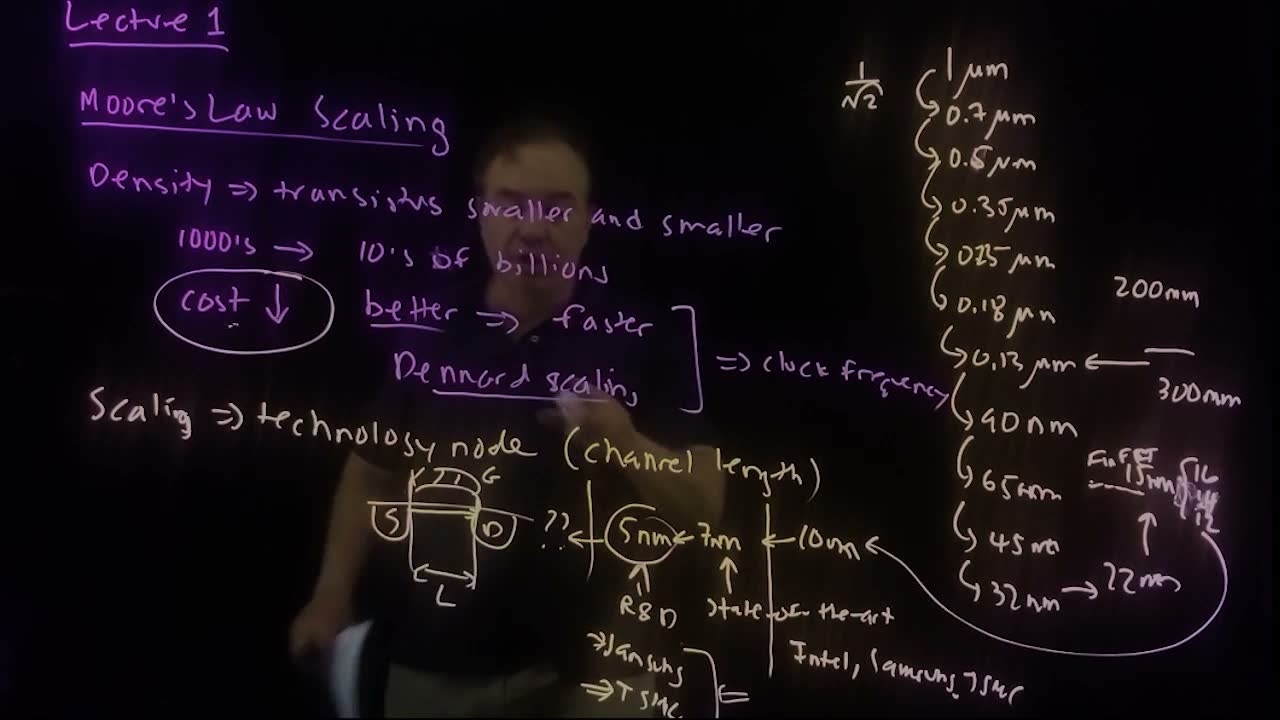
Moore’s law is named for Gordon Moore, a founder of Intel (9:51). added His 1965 paper was titled “Cramming more components onto integrated circuits”. It described the exponential growth in density of integrated circuits: transistors get smaller and smaller, and more and more of them fit on a chip.

• Density board: chips went from thousands of transistors to tens of billions (10:23). Designing something that large is a problem of its own, which Section 6 takes up.
• Cost board: the cost of each transistor has fallen with it. The lecturer recalls a comparison: one transistor costs less than one printed character in a copy of the New York Times, a tiny fraction of a cent (11:03–11:22).

The falling cost is the economic engine of Moore’s law (11:22). It is why the industry kept paying for each new generation, and Section 5 shows that cost is also what will end it.

Check yourself A chip with 10 billion transistors sells for about 100 dollars (an assumed price). What does one transistor cost?

100 dollars divided by $10^{10}$ is $10^{-8}$ dollars per transistor, that is $10^{-6}$ cents. That is even smaller than the lecture’s off-the-cuff “0.001 cents or something” (11:22): the point, a vanishingly small cost per transistor, holds with room to spare.

3. Smaller is also faster: Dennard scaling

The idea. Shrinking a transistor made it not only cheaper but better: faster. That bonus came free with each generation until it stopped.

The side benefit of scaling has a name: Dennard scaling, after Bob Dennard of IBM, who showed in a seminal paper how transistors get better as they shrink (11:52). “Better” means fundamentally faster (12:16): they switch faster, so a microprocessor’s clock frequency can rise. The board brackets “better ⇒ faster” and “Dennard scaling” together and points them at “clock frequency”.

Then the lecture states the bad news (12:26–12:53):

• the performance benefit has broken down. Shrinking no longer makes chips much faster;
• the cost benefit continues, so scaling continues;
• power, and more importantly power density (power per area), is the other half of the story.

Chapter 4 does all of this quantitatively: constant-field scaling shows why delay falls as $1/\kappa$ while power density stays constant, and the subthreshold slope shows why it broke.

Common mistakes.

• Treating Moore’s law and Dennard scaling as the same thing. Moore’s law is about density and cost; Dennard scaling is about speed and power. The second has ended, the first has (so far) not.
• Saying scaling has stopped. At the time of the lecture it was still going, for cost reasons (12:53).

Check yourself According to the lecture, which benefit of scaling has gone, and which remains?

The performance benefit (faster switching, higher clock frequency, the Dennard part) has largely gone. The cost benefit (cheaper transistors through density, the Moore part) remains, which is why scaling continues.

4. Technology nodes

The idea. A generation of technology, a node, is named after its shortest transistor dimension, the channel length. Each node shrinks lengths by about $1/\sqrt2$1/2​, which halves the area.

What a node names

A transistor has a source, a drain and a gate (13:39). Carriers, electrons or holes, travel from source to drain across the channel length $L$L. That is the length the board draws under the little transistor sketch.

Why you want $L$ short (14:07): the carriers move at a roughly fixed velocity, so a shorter path takes less time. The time to cross the channel is the transit time, and the shorter it is, the faster the technology.

So $L$ is made as short as the process can print: it is usually the critical dimension, the smallest feature the lithography can define (14:35). The node is named, roughly, by the channel length in that technology.

Worked example. added Lecture 5 makes “fixed velocity” precise: in a short channel the carriers cross at the saturation velocity $v_{sat} \approx 10^7\,\mathrm{cm/s}$107cm/s, so the transit time is $\tau_{tr} = L/v_{sat}$ (Chapter 5).

1. $L = 1\,\mu\mathrm{m} = 10^{-4}\,\mathrm{cm}$10−4cm: $\tau_{tr} = 10^{-4}/10^7 = 10^{-11}\,\mathrm{s} = 10\,\mathrm{ps}$10ps.
2. $L = 0.25\,\mu\mathrm{m}$0.25μm: four times shorter, so $\tau_{tr} = 2.5\,\mathrm{ps}$2.5ps.
3. $L = 65\,\mathrm{nm} = 6.5\times10^{-6}\,\mathrm{cm}$10−6cm: $\tau_{tr} = 0.65\,\mathrm{ps}$0.65ps.
4. Each node multiplies $L$L, and so $\tau_{tr}$τtr​, by about 0.71: about 1.4 times faster per node, as long as the velocity really stays fixed.

The node ladder

The lecture walks down the nodes from 1 µm, “probably around 1990 or so, maybe late 1980s” (15:02). The rule (15:30) is:

One technology nodeboard

$$L_{\text{next}} \approx \frac{L}{\sqrt2} \approx 0.7\,L$$$$A_{\text{next}} \approx \frac{A}{2}$$

The board writes only the $1/\sqrt2$1/2​. The area rule is spoken: each node halves the area per transistor, so the density doubles. Two nodes halve the length.

Holds when: the classic node sequence; the names after about 22 nm no longer follow it exactly

Multiply by $1/\sqrt2$ again and again added, and you get the node names on the board:

Step	$1\,\mu\mathrm{m}\times(1/\sqrt2)^n$	Node name	When (lecture’s recollection)
0	1 µm	1 µm	late 1980s / about 1990
1	0.707 µm	0.7 µm
2	0.5 µm	0.5 µm
3	0.354 µm	0.35 µm	about 1995
4	0.25 µm	0.25 µm	mid to late 1990s
5	0.177 µm	0.18 µm
6	0.125 µm	0.13 µm	wafers go from 200 mm to 300 mm
7	88 nm	90 nm	units change to nanometres
8	62.5 nm	65 nm
9	44 nm	45 nm
10	31 nm	32 nm
11	22 nm	22 nm
12	15.6 nm	16, 15, 14, 12 nm	FinFETs arrive
13	11 nm	10 nm
14	7.8 nm	7 nm	state of the art at the recording
15	5.5 nm	5 nm	in R&D at the recording

Points the lecture makes along the way:

• Microns to nanometres (16:52). After 0.13 µm the next node would have been “0.09 µm”; the industry switched units and called it 90 nm.
• Wafer size (17:08). Around the 0.13 µm node, silicon wafers grew from 200 mm to 300 mm in diameter. The board’s arrow points at 0.13 µm, the same node Lecture 2 gives (Chapter 2, Section 1).
• A “potpourri” of nodes after 22 nm (17:43). The rule predicts 15 nm, but depending on the foundry you find 16, 15, 14 and 12.
• FinFETs (18:10). Around this node the transistor changed shape: the gate now wraps around the channel (a fin). As planar transistors shrank, their electrostatics became very poor, and the new structure was needed to keep scaling going. Every node after this point uses FinFETs. Chapter 4 explains what “poor electrostatics” means for the subthreshold slope.
• 10, 7, 5 nm, and marketing (18:38–19:43). At the smallest nodes every foundry uses slightly different names, and the “critical dimension” has become vague (drawn versus actual dimensions). The node name is now “almost more of a marketing play”. At the recording, 7 nm was the state of the art and R&D worked at 5 nm; the board’s “??” marks what comes after.

added This term’s design work uses TSMC’s 65 nm planar bulk process, and introduces TSMC’s 16 nm FinFET process (N16). Both sit on the board’s ladder, on either side of the FinFET switch.

Check yourself How many 1/√2 steps take 1 µm to 5 nm, and by how much does the area per transistor shrink?

The ratio is $1000/5 = 200$200, and $\ln 200/\ln\sqrt2 = 15.3$15.3, so about 15 nodes, as the ladder shows. The area shrinks by $200^2 = 40{,}000$ (or $2^{15} \approx 33{,}000$ counting nodes). Keep in mind that the names below about 22 nm are no longer true lengths.

Check yourself The lecture's ladder runs from 1 µm around 1990 to 5 nm in R&D at the recording, about 2020. How often did a new node arrive?

About 30 years for 15 nodes: one node every two years or so. added That matches the usual statement of Moore’s law, density doubling about every two years, since each node doubles the density.

Common mistakes.

• Shrinking the length by half per node. It is $1/\sqrt2$ per node; it is the area that halves.
• Reading “5 nm” as a physical 5 nm channel. Below about 22 nm the names are labels, not measurements.

5. Who can still afford to scale

The idea. Each new node needs a new factory costing billions of dollars, so fewer and fewer companies can keep up. In the end, economics, not physics, will stop scaling.

Building a fab at the leading nodes costs billions of dollars (20:19). As the cost rose, the number of companies that could follow dropped (20:47–21:45):

• at the older nodes, perhaps 20 or 30 foundries built leading-edge chips;
• Texas Instruments and then GlobalFoundries dropped out;
• at about 10 nm, three were left: Intel, Samsung and TSMC board;
• Intel was struggling at 7 nm, and at 5 nm only two remained: TSMC (Taiwan Semiconductor Manufacturing Company) and Samsung Electronics (Korea).

What will end scaling? Economics (22:19). Scaling stops when the benefit, a cheaper transistor, is no longer worth the cost and difficulty of the next node. The lecturer argues “we’re getting very, very close to that point now”.

How the two survivors pay for it (22:48–23:16): TSMC builds chips for many companies, with Apple and Qualcomm the biggest customers, and so uses economies of scale. Samsung uses the volume of its own mobile-phone business, and also does foundry work for others.

Check yourself Why does the lecture expect economics, rather than physics, to end scaling?

Because scaling has always been paid for by the cheaper transistor it delivers. Each node now costs billions and is harder to make; when the cost reduction no longer pays for that, nobody will build the next node, whatever physics allows.

6. Levels of abstraction

The idea. Nobody can reason about ten billion transistors at once. Engineers describe the chip at several levels, each hiding the details of the one below, and work at whichever level suits the question.

At the bottom it is all physics (25:50): electrons and holes in a crystal, drift and diffusion, electrostatics. In principle the whole microprocessor could be understood that way; in practice the complexity would be unmanageable. So we build levels of abstraction: when the details don’t matter, we stop looking at them (26:15).

Lecture01 @ 37:37The levels of abstraction, bottom (devices) to top (system), with the tools between them. The lecturer stands over 'Circuits'.

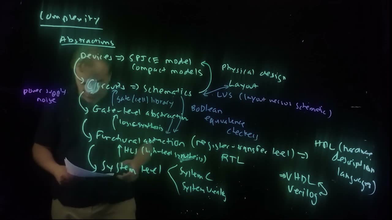
From the bottom up (26:27–32:33) board:

Level	How it is described	What it hides
Devices (transistors)	SPICE models, also called compact models: equations for current, voltage and capacitance	the drift–diffusion and electrostatics underneath
Circuits	schematics: circuit diagrams of interconnected devices	individual device physics
Gate level	logic gates (NAND, NOR), flip-flops, memory cells	transistors
Functional (RTL)	a register-transfer level description, written in an HDL	individual gates
System level	higher-level languages such as SystemC and SystemVerilog	the state elements

A few notes on each:

• SPICE is named after the original circuit-simulation program. Device engineers say compact models, because the equations are far more compact than solving drift and diffusion directly (26:58–27:43). Lectures 2–5 build the simplest such models by hand. added The lecture dates SPICE to the 1980s; it was in fact released at UC Berkeley in the early 1970s.
• RTL (29:10). Every register, every state element, is explicitly present, and the description shows how information moves from register to register through logic each clock cycle. It is written in a hardware description language (HDL).
• The two common HDLs (30:23–31:07). VHDL came out of a government standardization project. Verilog was proprietary at Cadence; competition from VHDL forced Cadence to open it to the public, and the two have coexisted since. Most CAD tools accept both. added Verilog was created at Gateway Design Automation, which Cadence bought in 1989.
• System level (31:44). Functional descriptions that need not spell out every state element. SystemVerilog extends Verilog, and SystemC extends the C language.

This course uses HDLs only a little; other courses use them heavily (31:21).

Physical design sits beside these levels (32:44–33:24): the layout, the actual shapes printed on the chip.

Which level to use depends on the question. To study a processor’s microarchitecture and its interaction with software, you would never work at the device level (32:33). But at every level you must be able to check that the design is right.

Check yourself At which level is a flip-flop a single block, and at which is it a set of transistors?

At the gate level a flip-flop is one element, like a NAND gate. At the circuit level (a schematic) it is its transistors and their connections.

7. Tools that move between the levels

The idea. CAD (computer-aided design) tools either generate the next level down automatically or check that two levels agree.

The board’s arrows (33:24–35:30):

Tool	From → to	Generates or checks
High-level synthesis (HLS)	system level → RTL	generates
Logic synthesis	RTL → gate level	generates
Gate (cell) library	gate level → circuits: a schematic for every gate	provides
Boolean equivalence checker	gates or schematics against the RTL	checks
LVS, layout versus schematic	layout against the schematics	checks

These tools are how the complexity is managed (35:30). The course’s designs are far smaller than ten billion transistors, but the same ideas apply.

added In this term’s lab, LVS is run with Mentor Calibre (syllabus).

Check yourself A layout passes LVS. Does that prove the chip computes the right function?

No. LVS only shows the layout matches the schematic. Whether the schematic implements the RTL is a separate check (a Boolean equivalence checker), and whether the RTL is what you wanted is yet another question.

8. Problems that cross the levels

The idea. Abstraction compartmentalizes most work, but some of the hardest problems cut through every level at once.

The lecture’s main example is power-supply noise (36:25–37:28). When circuits switch, they draw current from the chip’s power grid, and the supply voltage fluctuates briefly. That changes how every circuit behaves. How much noise there is depends on what the processor is doing, so it depends on the software and the system level. Yet it is a deeply physical effect at the circuit and device level. To understand it you must work across the levels.

Other examples (37:28–37:38): coupling noise between wires, clocking, testing and reliability. These are among the most challenging problems in designing a modern microprocessor (37:38).

Check yourself Why can't power-supply noise be understood at the circuit level alone?

Because how much current the circuits draw, and when, depends on what the processor is doing: the software and the system-level activity. The effect itself is physical (the supply grid’s voltage sagging), so you need both ends of the abstraction stack.

9. Analog versus digital

The idea. Every circuit is analog. “Digital” is a way of using analog circuits, with two well-separated voltage levels, that makes them immune to noise and tolerant of variability.

Lecture01 @ 51:01Analog versus digital (left) and semiconductor technologies (right).

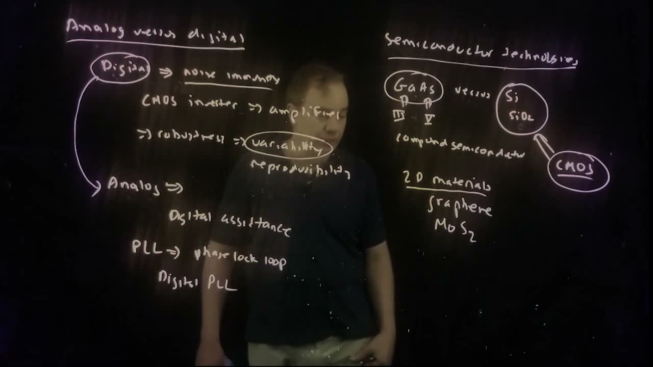
Designers call themselves analog, digital or mixed-signal designers (39:17). But all circuits are analog (39:40): they work with continuous voltages, continuous currents and continuous time. What makes a circuit digital is how it is used (39:53):

• it is switched between two voltages, rail to rail;
• the voltages are abstracted into two states, separated by noise margins (40:21). A signal disturbed by noise is still read as the right state, as long as the noise stays within the margin.

The classic example is the CMOS inverter (40:30). It is nothing more than an analog amplifier; the way we use it is what makes it digital. Its noise margins come in the CMOS-inverter lecture (Lecture 6).

What digital buys board (40:51–42:17):

• noise immunity;
• robustness to variability: devices vary because of process variations, and a digital circuit works anyway;
• reproducibility: two copies of the same circuit behave alike, because they are easy to make work the same way.

These matter more and more as nodes shrink, because deeply scaled processes have a lot of process variability (41:50). Chapter 3 shows one cause, random dopant fluctuations.

Why analog is still needed (42:17–43:30). Some functions are inefficient in digital form, in power or in performance. A radio receiver is the example: the antenna signal is in the gigahertz range. Converting it straight to digital would need a data converter that burns an enormous amount of power, and the digital processing would be very inefficient too. Instead you amplify it in analog, mix it down to a lower frequency, and only then convert it.

The price (43:30–44:08). Analog circuits lack digital’s protections: they are sensitive to variability, not very reproducible, and sensitive to noise. That is why analog design is often thought to be harder.

Check yourself The lecture calls a CMOS inverter 'nothing more than an analog amplifier'. What, then, makes it a digital gate?

How it is used: its input and output are driven between the two rails and read as one of two states, separated by noise margins. The amplifier’s gain is what restores a noisy input to a clean output level.

Common mistakes.

• Thinking digital circuits are a different kind of physics. They are the same transistors, with the same continuous voltages; only the use differs.

10. Digital helping analog

The idea. Digital circuits increasingly correct the weaknesses of analog ones, and some analog functions have moved into digital entirely.

• Digitally assisted analog (44:08–44:27): digital circuits measure and correct the imperfections of the analog circuits next to them.
• From analog to digital (44:27–45:59). If a function once done in analog can be done digitally, that has enormous advantages. The best example is the PLL, the phase-locked loop. In a microprocessor a PLL generates the clock, typically multiplying a lower-frequency reference up to a higher on-chip frequency. PLLs were analog circuits until recently; now there are digital PLLs, designed largely with digital tools such as synthesis, almost as a logic description.

Does that mean analog is going away? “Of course nonsense” (45:59): many functions will always be analog. Digital is there to help.

Check yourself What is the lecture's best example of a function moving from analog to digital, and what does the move buy?

The phase-locked loop. A digital PLL can be designed largely with digital tools such as synthesis, almost as a logic description, and so gains digital’s robustness to variability and noise.

11. Why silicon

The idea. Other semiconductors have better raw properties than silicon, but silicon has a native oxide and CMOS scaling. Silicon CMOS won and will keep winning.

Gallium arsenide (46:44–48:03) is a III–V material: gallium is in group III of the periodic table and arsenic in group V board. It is a compound semiconductor; silicon, a single element, is an elemental semiconductor (49:07). In the 1980s GaAs was widely touted as silicon’s replacement, because it has a higher low-field mobility (Chapter 4 defines mobility). But it had serious problems:

• no native oxide. Gallium does oxidize, but the oxide dissolves in water, a big problem for processing;
• silicon has one: SiO₂ board, which gave silicon a lot of advantages. Chapter 3’s MOS capacitor is built on it.

What happened (48:03–49:34). III–V materials (GaAs, indium phosphide, indium arsenide) never displaced silicon for integrated circuits. They found two homes:

• optoelectronics, such as LEDs, where their direct band gap lets them emit light. Silicon’s band gap is indirect, so it is a poor light emitter;
• niche microwave applications. Even there, CMOS kept getting faster with scaling and took over many of these circuits.

At short channel lengths, low-field mobility matters less anyway (49:34). The current is then limited by other things, such as the source injection velocity, which erased much of GaAs’s advantage. Chapter 4 meets this as velocity saturation.

2D materials (50:09–51:29), crystals only one or a few atomic layers thick, are the newer candidates: graphene and MoS₂ (molybdenum disulfide). The physics is very interesting, but graphene has no band gap, so it can’t switch off, and MoS₂ is inferior to silicon in many respects. The lecturer remains “deeply skeptical” that they will ever matter for electronics.

The takeaway (51:03–51:29): silicon CMOS has enormous advantages and will rule for the foreseeable future. As scaling ends, performance gains will have to come from the system level, not from the underlying technology.

Check yourself Give the lecture's two reasons silicon beat gallium arsenide for integrated circuits, despite GaAs's higher mobility.

(1) Silicon has a stable native oxide, SiO₂; gallium’s oxide dissolves in water. (2) CMOS scaling kept improving silicon, and at short channel lengths the low-field mobility advantage matters much less.

12. MOS versus BJT

The idea. The bipolar transistor came first and once ran the fastest computers, but it burns too much power. CMOS replaced it for logic.

Lecture01 @ 55:18MOS versus BJT, with the ECL mainframe's 2 ns cycle. The arrow from BJT back to MOS is IBM's move to CMOS. The left half is mid-erasure.

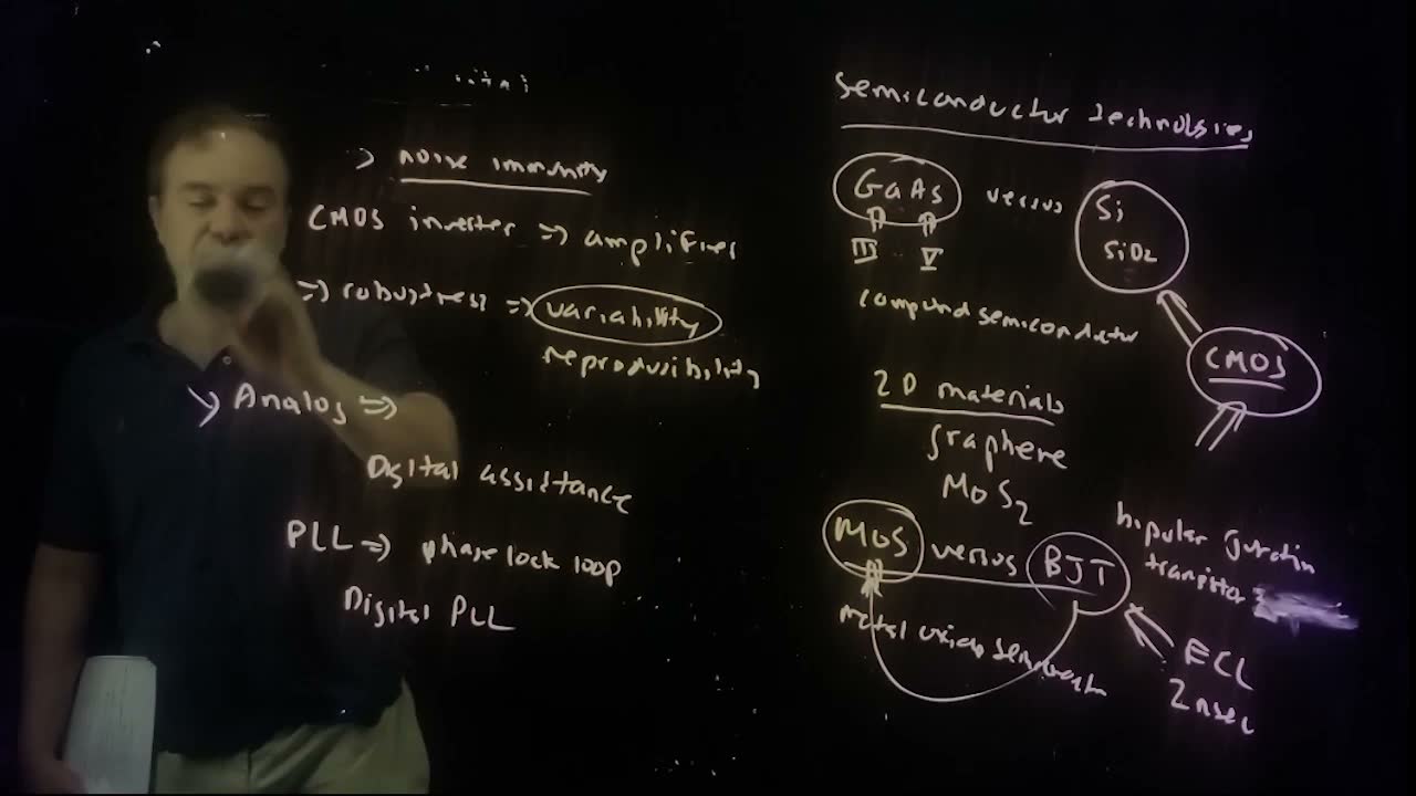
There are two kinds of transistor (51:29):

• the BJT, bipolar junction transistor, invented at Bell Labs in the 1940s, work that received the Nobel Prize (51:59–52:11). added Strictly, the very first transistor (1947) was a point-contact transistor; Shockley’s junction transistor followed in 1948. The 1956 Nobel Prize went to Shockley, Bardeen and Brattain for the transistor;
• the MOS transistor, metal–oxide–semiconductor, developed after it (52:18). Chapter 3 introduces its structure.

For digital circuits, MOS has come to dominate (52:30).

The bipolar mainframes (52:30–54:44). Until about 1992, all high-end computers, such as IBM’s mainframes, used bipolar logic. The circuit style was ECL, emitter-coupled logic board: a current-steering logic, in which a current is steered one way or the other to represent the logic state.

Worked example. added The lecture’s numbers for one such machine.

1. Cycle time 2 ns board: clock frequency $f = 1/(2\times10^{-9}\,\mathrm{s}) = 5\times10^8\,\mathrm{Hz} = 500\,\mathrm{MHz}$500MHz, “extremely fast” for its day (53:19).
2. One processor took 121 chips, each dissipating about 100 W (53:32).
3. Total: $121 \times 100\,\mathrm{W} = 12.1\,\mathrm{kW}$12.1kW, the lecture’s “about 12 kilowatts” for one microprocessor (54:03).

The chips sat in thermal conduction modules: copper pistons pressed against the back of each chip, into a heat sink with chilled water flowing in on one side and “boiling water” coming out the other (53:32). One module cost tens of thousands of dollars, perhaps 100,000 dollars. Bipolar logic was power-hungry, needed expensive packaging and didn’t scale well (54:11). In about 1992 IBM switched its mainframes to CMOS, and since then CMOS has been the dominant technology for microprocessors (54:44).

Check yourself Why did one bipolar processor need 121 chips, while a CMOS chip today holds billions of transistors?

Bipolar logic burned so much power per gate (current always flowing in ECL) that only a limited amount of logic could be packed and cooled on each chip, and it didn’t scale well. CMOS draws little power when not switching and kept scaling, so density could grow by many orders of magnitude.

13. Coming next: the device-physics road map

The idea. A circuits course needs device physics, because circuits are built from devices. The next four lectures go through it quickly, and this outline is their table of contents.

The lecturer makes “no apologies” for the device physics (56:17): understanding how devices work is essential to designing circuits, and it goes quickly for those who have seen it.

Lecture01 @ 60:05The device-physics outline for Lectures 2 onward.

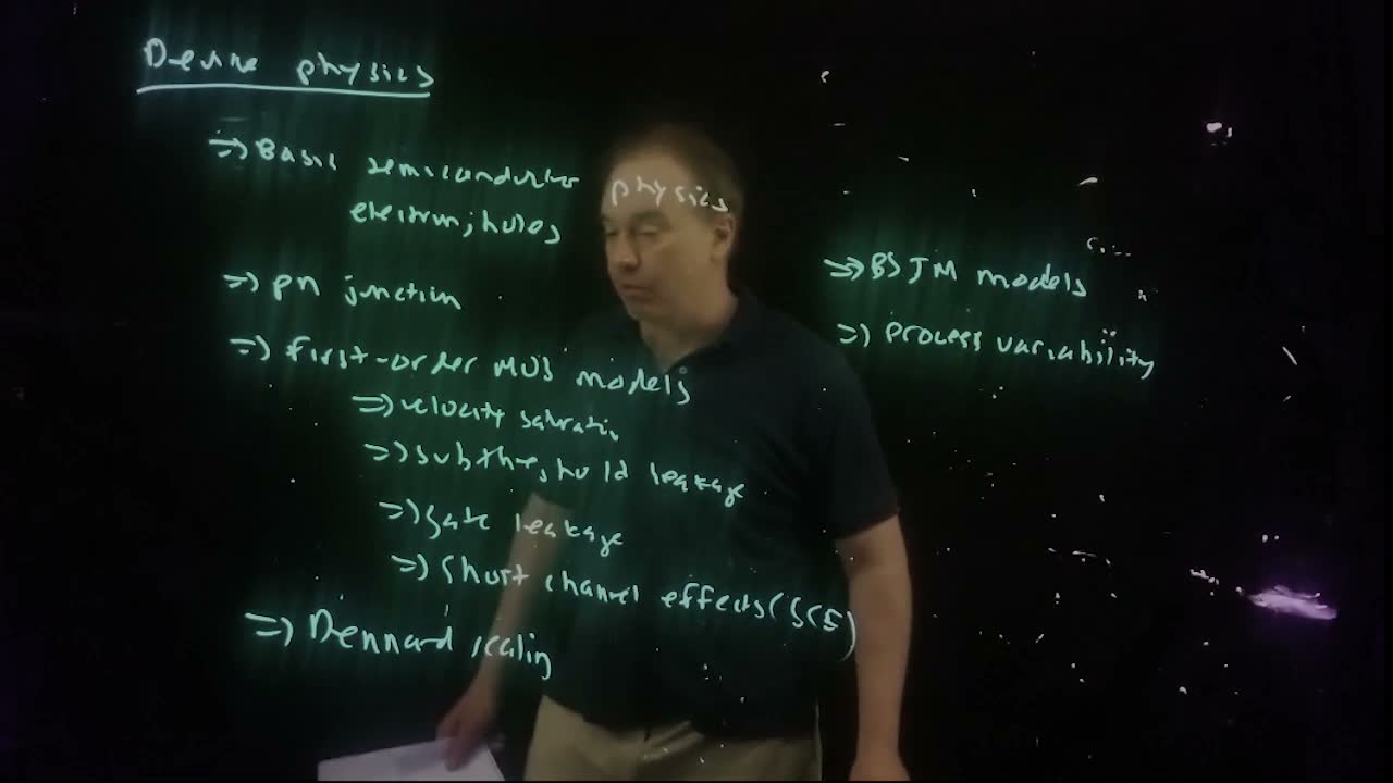
Much of the basic semiconductor physics was developed at Bell Labs by William (Bill) Shockley (57:04), who shared the Nobel Prize for the transistor. He later left for California and founded his own transistor company, recruiting some of the people who started the semiconductor industry there: Silicon Valley is in the San Francisco Bay Area because of him (57:40–58:07). His book, Electrons and Holes in Semiconductors (1950), underlies the physics the course uses.

The outline board, and where this guide covers it:

Board item	Where
Basic semiconductor physics: electrons, holes	Chapter 2
pn junction	Chapter 2 and Chapter 3
First-order MOS models (the Shockley long-channel model)	Chapter 3 (threshold) and Chapter 4 (I–V)
Velocity saturation	Chapter 4
Subthreshold leakage	Chapter 4
Gate leakage	Chapter 4
Short-channel effects (SCE)	Chapter 4
Dennard scaling, and why it broke	Chapter 4
BSIM models, the most common compact models today	later lectures (Batch 2)
Process variability: causes, modelling	Chapter 3 (random dopants); more later

The lecture introduces the long-channel model first and then shows “how it doesn’t work” (58:46): each item under it is a way real, short transistors depart from it.

Numbers to remember

Rule or number	Meaning
$L_{\text{next}} \approx L/\sqrt2 \approx 0.7L$	one technology node
$A_{\text{next}} \approx A/2$	area per transistor halves; density doubles per node
1, 0.7, 0.5, 0.35, 0.25, 0.18, 0.13 µm; 90, 65, 45, 32, 22 nm; then 16/14, 10, 7, 5 nm	the node ladder; FinFETs from about 16/14 nm
$\tau_{tr} = L/v_{sat}$	transit time across the channel: shorter $L$L, faster (Chapter 5)
$f = 1/T$	clock frequency from cycle time: 2 ns ↔ 500 MHz
devices → circuits → gates → RTL → system	levels of abstraction; layout beside them
HLS, logic synthesis; equivalence checking, LVS	tools that generate, and tools that check

The lecture’s boards

Lecture01 @ 23:43 Moore's law, Dennard scaling, the node ladder

Lecture01 @ 37:37 levels of abstraction and CAD tools

Lecture01 @ 51:01 analog versus digital; semiconductor technologies

Lecture01 @ 55:18 MOS versus BJT, ECL at 2 ns

Lecture01 @ 60:05 the device-physics outline