17. Prefix adders and shifters: radix-2 trees, shifters and control logic

Lecture 16 finishes the adders and moves on to the other datapath blocks. Chapter 16 ended with a radix-4 lookahead tree. This lecture builds trees out of the smallest possible block, the radix-2 element, which merges two adjacent groups of bits into one. Because the element is associative, the carries can be computed by many different networks of it. The lecture draws the two classic ones, Kogge–Stone and Brent–Kung, and compares them: the first is fast and regular, the second small. The textbook name for these adders is prefix adders, because every carry turns out to be a prefix of the row of bits. The lecture then turns to shifters: the three kinds of shift, the logarithmic shifter built from rows of multiplexers, and the barrel shifter built from a grid of pass transistors with a one-hot select. It ends with control logic: why it is synthesized, how the synthesis and place-and-route flow runs, and why the course builds its control logic as a PLA instead (Chapter 18).

After this chapter you can:

1. combine two adjacent groups with the radix-2 element, in the right order, and say why any bracketing works;
2. say which group each carry and each sum needs, with the carry-in entered as $(c_{in}, 0)$(cin​,0);
3. draw the Kogge–Stone and Brent–Kung networks for a given width and count their elements, levels and fan-outs;
4. say which is faster and which is smaller, and why;
5. draw a complete prefix adder (PG cells, network, sums) and its critical path;
6. shift a word logically, arithmetically and by rotation, and explain sign extension;
7. build a logarithmic shifter from 2:1 multiplexers, logical or arithmetic, and find its stack height;
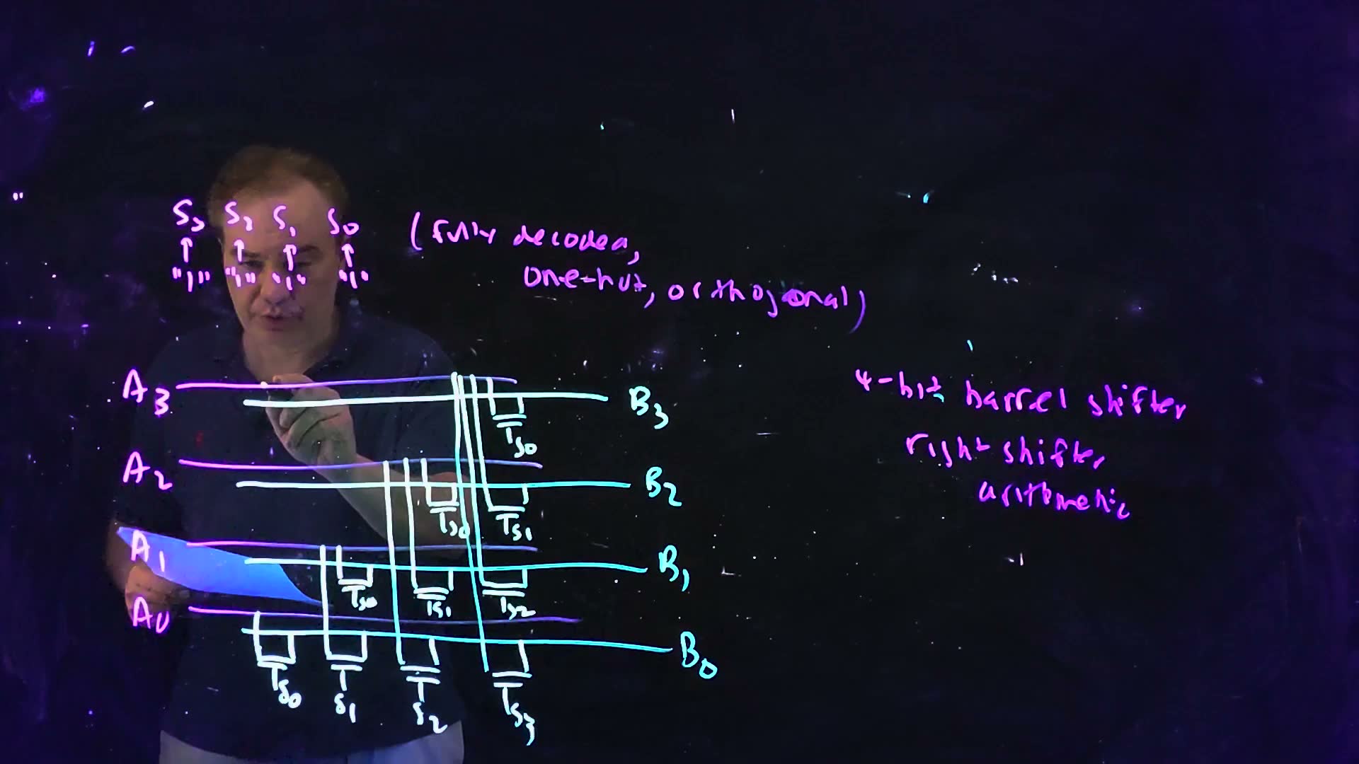
8. build a barrel shifter from pass transistors and explain why its select must be one-hot;
9. describe the two ways to build control logic and the synthesis and place-and-route flow;
10. say what a PLA implements (two-level sum-of-products logic) and where Chapter 18 takes it up.

Boxes and equations marked board were written in the lecture. Parts marked added are explanations, arguments or examples this guide adds; every number in them is recomputed in the page’s test.

Before you start. Chapter 16 built the pieces this chapter assembles. Each bit of an adder has a PG cell that makes its generate $g = ab$ (the bit makes a carry by itself) and its propagate $p = a\oplus b$ (the bit passes an incoming carry on); the bit’s carry out is $g + p\,c_{in}$ and its sum is $p\oplus c_{in}$ (Chapter 16, §9). A group of bits behaves like one big bit, with a group generate $G$ and group propagate $P$P, and two adjacent groups merge into one by the radix-2 element (Chapter 16, §12). A lookahead tree computes the carries in a number of steps that grows with $\log N$logN, not $N$ (Chapter 16, §13). Delays are counted in levels, the number of elements a signal passes in series, as Chapter 16 counted lookahead units. Where a delay is given in $\tau_{inv}$ (the fan-out-of-one inverter delay, the course’s unit), it uses example values, labelled “for example”: a PG cell $t_{PG} = 2$2, a sum XOR $t_{sum} = 4$ (Chapter 16’s) and one element $t_e = 4\,\tau_{inv}$4τinv​, the same as one carry stage, since an element’s $G_{hi} + P_{hi}G_{lo}$ is the carry stage’s $g + p\,c_{in}$ one level up.

Bit numbering. This chapter numbers the bits from 1, as the board and FN17-8 do, with the carry-in at position 0. Chapter 16 numbered them from 0. The carry wires keep their names: $C_k$ here, the carry out of bit $k$k, is the same wire as Chapter 16’s $c_k$ck​. The sum’s index shifts: here $s_k = p_k\oplus C_{k-1}$Ck−1​, there $s_i = p_i\oplus c_i$ci​.

Symbols

Symbol	Meaning	Unit	First appears
$a_k$ak​, $b_k$	bit $k$ of the two operands, $k = 1 \dots N$1…N; bit 1 is the least significant (the board’s and FN17-8’s numbering; Chapter 16’s bit $k - 1$1)	—	§2
$c_{in}$cin​, $c_{out}$	the adder’s carry in (position 0) and carry out ($c_{out} = C_N$cout​=CN​)	—	§1, §2
$g_k$gk​, $p_k$	generate $a_kb_k$ and propagate $a_k\oplus b_k$ of bit $k$ (Chapter 16 §9)	—	§1
$(g, p)$(g,p), $(g', p')$	the board’s names for the element’s two inputs: unprimed the higher group, primed the lower	—	§1
$G_{i:j}$Gi:j​, $P_{i:j}$	group generate and propagate of positions $j$ to $i$i, high index first; the board writes the span low–high, “$j$j–$i$i”	—	§1
$(G_{hi}, P_{hi})$(Ghi​,Phi​), $(G_{lo}, P_{lo})$	the element’s higher and lower inputs in the chapter’s form	—	§1
$\circ$	the radix-2 element (the circle drawn inside the board’s box)	—	§1
$(c_{in}, 0)$	the carry-in entered as a group of its own at position 0: it generates when $c_{in} = 1$ and propagates nothing	—	§1, §2
$C_k$	$G_{k:0}$Gk:0​, the carry out of bit $k$ (the board’s $C_1 \dots C_8$C1​…C8​); the same wire as Chapter 16’s $c_k$	—	§2
$s_k$	sum bit $k$k: $s_k = p_k\oplus C_{k-1}$Ck−1​, with $C_0 = c_{in}$	—	§2
$N$	the number of bits (§2–§4) or of positions (§5); the number of bits of a shifter (§8–§9)	—	§2
level	one element on a signal’s path; a network’s depth is its number of levels	—	§2
$t_e$te​, $t_{PG}$tPG​, $t_{sum}$	the delays of one element added, one PG cell and one sum XOR (Chapter 16)	$\tau_{inv}$	§5
$\tau_{inv}$	the fan-out-of-one inverter delay, the unit of delay	ps	§5
KS, BK	Kogge–Stone, Brent–Kung	—	§3, §4
MSB, LSB	the most and least significant bits of a word	—	§7
$A_i$	bit $i$ of a shifter’s input word, $A_0$ the LSB (the board’s $A_7 \dots A_0$A7​…A0​)	—	§7
$Y_i$	bit $i$ of the logarithmic shifter’s output	—	§8
$S_k$	a select bit: encoded $S_2S_1S_0$ in the logarithmic shifter (§8); one-hot $S_0 \dots S_3$ in the barrel shifter (§9)	—	§8
sel, $\overline{\text{sel}}$	a 2:1 multiplexer’s select and its complement	—	§8
$B_j$	bit $j$ of the barrel shifter’s output	—	§9
stack height	the number of devices a signal’s charge passes in series, its driver included	—	§8
RTL, SOP, PLA, P&R, STA, GDS	register-transfer level; sum of products; programmable logic array; place and route; static timing analysis; the layout file that goes to the foundry	—	§10

1. The radix-2 element and why its order matters

You need

Generate and propagate (Chapter 16, §9). One bit with operands $a$a, $b$ has $g = ab$ and $p = a\oplus b$b. If $g = 1$1, the bit makes a carry whatever comes in; if $g = 0$ and $p = 1$1, it passes its incoming carry through; if both are 0 it kills the carry. Its carry out is $c_{out} = g + p\,c_{in}$pcin​.

Groups (Chapter 16, §12). A run of bits behaves like one big bit: its carry out is $G + P\,c_{in}$Pcin​. For two bits, $G = g_1 + p_1g_0$ (bit 1 generates, or bit 0 generates and bit 1 passes it) and $P = p_1p_0$ (both pass).

Chapter 16’s radix-2 element (§12): two adjacent groups make one. Original figure ↗

The question. A tree adder needs one small block it can repeat everywhere. What is the smallest block that merges the carry information of two groups, and what rules must a tree of such blocks follow?

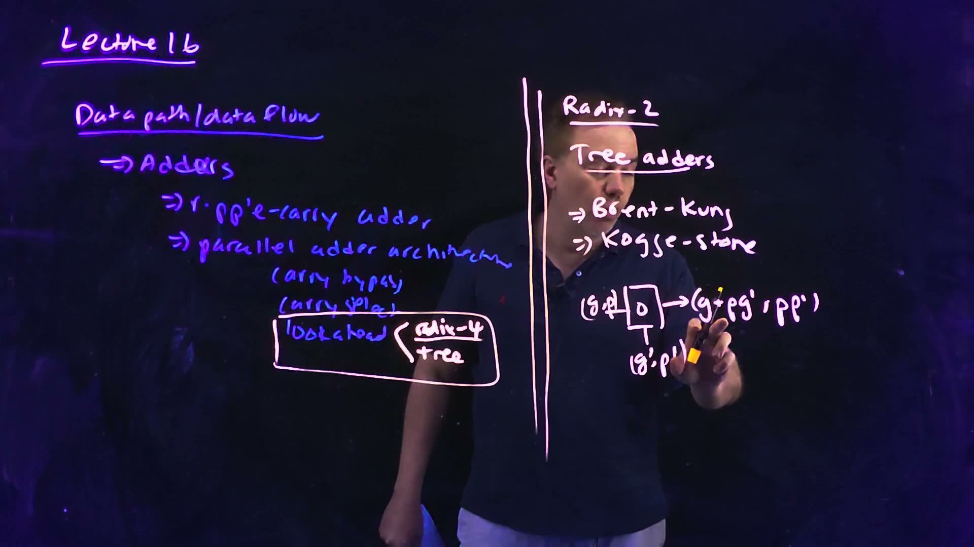
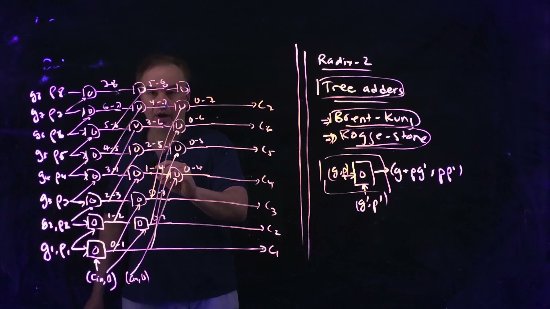
The element (board, 00:53–03:32)

1. Where we are (00:53–02:03) board. The lecture opens with a recap: the ripple-carry adder, then the parallel architectures, carry bypass, carry select and the radix-4 lookahead tree. Today, radix-2 trees: “Brent–Kung” and “Kogge–Stone” (both ringed on the board at 03:32).
2. The block (02:03–02:47) board. A square box with a small circle inside. A pair $(g, p)$ enters from the left, a pair $(g', p')$ from below, and $(g + pg',\ pp')$ leaves on the right. Read it as Chapter 16’s two-bit group with groups in place of bits: the left input is the higher group, the primed input from below the lower one. The output generates if the higher group generates, or if the lower group generates and the higher group passes it on; it propagates only if both do.
3. Spans added. Name a group by the positions it covers, high index first: $G_{i:j}$ and $P_{i:j}$ cover positions $j$ to $i$i. The element merges two spans that touch, the higher on the left: $(G_{i:j}, P_{i:j}) = (G_{i:k}, P_{i:k})\circ(G_{k-1:j}, P_{k-1:j})$(Gk−1:j​,Pk−1:j​). In the chapter’s form, $(G_{hi}, P_{hi})\circ(G_{lo}, P_{lo}) = (G_{hi} + P_{hi}G_{lo},\ P_{hi}P_{lo})$Phi​Glo​, Phi​Plo​).
4. Associativity (02:47–03:10). The lecturer’s key claim: “I can combine them and associate them in any way I choose … and ultimately you get the same answer” (03:00). Three adjacent groups $x$x, $y$y, $z$ (highest first) give the same result whether $x$ and $y$ are merged first or $y$ and $z$z. The derivation is below.
5. Not commutative added. The two inputs cannot be swapped. A killing high group, $(0, 0)$(0,0), over a generating low group, $(1, 0)$(1,0), gives $(0,0)\circ(1,0) = (0 + 0\cdot1,\ 0) = (0, 0)$(0,0): the carry made below is killed above it. Swap them and $(1,0)\circ(0,0) = (1, 0)$(1,0): a carry appears that the real bit order never makes. Of the nine ordered pairs of possible inputs ($(1, 1)$(1,1) cannot occur, since a bit’s $g = ab$ and $p = a\oplus b$ are never both 1, and a group’s $P = 1$ means no bit in it generates), two change when swapped: exactly the kill-over-generate pair of this example, in either order. Bracket as you like; never swap.

The radix-2 element as the board draws it (Lecture16 @ 03:32). The higher group $(g, p)$ enters from the left, the lower group $(g', p')$ from below, and the element returns $(g + pg',\ pp')$pg′, pp′). The second line under each label is the chapter’s form: $(G_{hi}, P_{hi})\circ(G_{lo}, P_{lo}) = (G_{hi} + P_{hi}G_{lo},\ P_{hi}P_{lo})$Phi​Glo​, Phi​Plo​).

The board (Lecture16 @ 03:32)

Lecture16 @ 03:32The recap, and the radix-2 element: (g, p) ∘ (g′, p′) = (g + pg′, pp′).

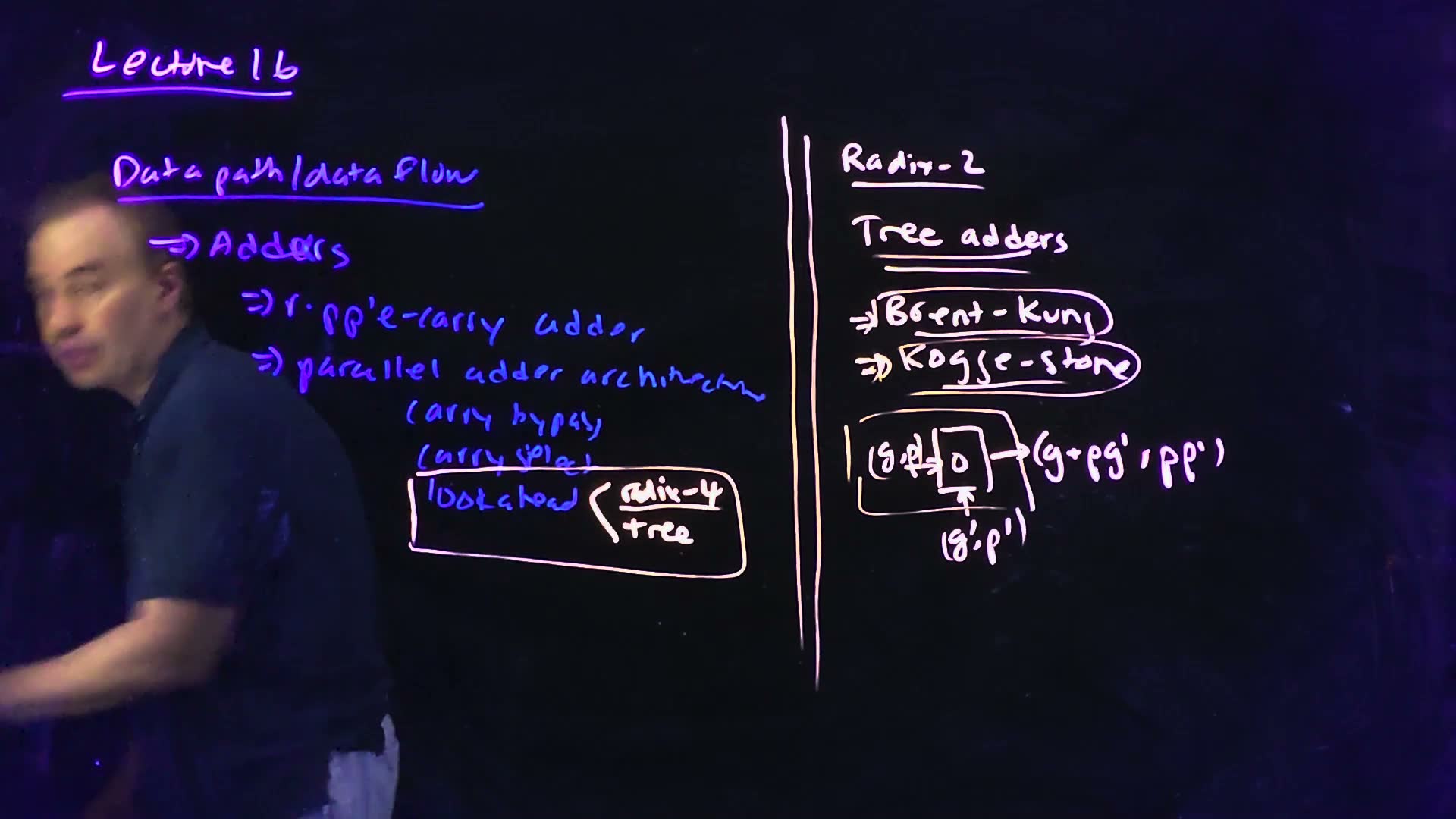
Fair copy of the board above (Lecture16 @ 03:32), mark for mark in its own layout. All black: the violet pen wrote the recap at the left, from “Lecture 16” to “lookahead”; the cream pen wrote the double rule and the right half, the next topic, and boxed “lookahead” on the recap with its branch to “radix-4” and “tree”. The board writes “ripple” with its i shrunk to a dot and its l to a tick; it is set in full. “architectures” trails off after “architec” into a squiggle, copied as it stands.

Any two adjacent spans merge in one element added: the higher span 8:5 enters from the left, the lower span 4:0 from below, and the result is the span 8:0, $G_{8:0} = G_{8:5} + P_{8:5}G_{4:0}$ (and $P_{8:0} = P_{8:5}P_{4:0}$P8:5​P4:0​). Position 0 is the carry-in.

The radix-2 elementboard

$$(G_{hi}, P_{hi})\circ(G_{lo}, P_{lo}) = (G_{hi} + P_{hi}G_{lo},\ P_{hi}P_{lo})$$

Holds when: the two inputs are adjacent spans, the higher one first (on the board, the left input); the order cannot be swapped

Memorize or derive. Memorize the element: it is FN17-8’s “radix-two lookahead element”, $G = g_1 + p_1g_0$p1​g0​, $P = p_1p_0$p1​p0​, with groups for bits. Derive associativity added by expanding both bracketings of three groups $x$x, $y$y, $z$ (highest first):

$$\begin{aligned} (x\circ y)\circ z &= (g_x + p_xg_y,\ p_xp_y)\circ(g_z, p_z)\\ &= (g_x + p_xg_y + p_xp_yg_z,\ p_xp_yp_z)\\ x\circ(y\circ z) &= (g_x, p_x)\circ(g_y + p_yg_z,\ p_yp_z)\\ &= (g_x + p_xg_y + p_xp_yg_z,\ p_xp_yp_z) \end{aligned}$$

Both are “a carry made in $x$x, or made in $y$ and passed by $x$x, or made in $z$ and passed by $x$ and $y$y”: the same group. That is what lets a tree replace the chain: any bracketing of the same bits in the same order gives the same carry.

A worked example added. Bits 3, 2, 1 with $(g, p) = (0, 1)$(0,1), $(1, 0)$(1,0), $(0, 1)$(0,1): bit 3 passes, bit 2 generates, bit 1 passes. Bracketed from the top, $((0,1)\circ(1,0))\circ(0,1) = (0 + 1\cdot1,\ 1\cdot0)\circ(0,1) = (1,0)\circ(0,1) = (1, 0)$(1,0). Bracketed from the bottom, $(0,1)\circ((1,0)\circ(0,1)) = (0,1)\circ(1 + 0\cdot0,\ 0\cdot1) = (0,1)\circ(1,0) = (1, 0)$(1,0). Both say the group 3:1 generates a carry and does not propagate one: bit 2 makes the carry and bit 3 passes it, and bit 2’s $p = 0$ blocks any carry from below.

Traps.

• Putting the lower group on the left. The result is the group of a different bit order; the counter-example in step 5 shows it can invent a carry.
• Reading the board’s primes as “later” or “the output”. They mark the lower group, nothing else.

Check yourself What (G, P) does a group have whose every bit propagates (each g_k = 0, p_k = 1)?

$(0, 1)$(0,1): no bit generates, so the group makes no carry of its own, and every bit passes, so it passes its carry-in through. Merging two such groups gives $(0 + 1\cdot0,\ 1\cdot1) = (0, 1)$ again.

Check yourself Combine a group (G_hi, P_hi) with the carry-in entered as (c_in, 0) below it. What comes out, and what is it?

Step 1: $(G_{hi}, P_{hi})\circ(c_{in}, 0) = (G_{hi} + P_{hi}c_{in},\ P_{hi}\cdot0) = (G_{hi} + P_{hi}c_{in},\ 0)$Phi​cin​, 0). Step 2: the first half is Chapter 16’s group carry, $c_{out} = G + P\,c_{in}$Pcin​: the group’s carry out with this carry-in. The propagate is 0 because the carry-in is already inside the span; nothing below it is left to pass on.

2. Every carry is a prefix: the serial chain

You need

The element and its order (§1). Two adjacent spans merge, the higher on the left: $(G_{hi}, P_{hi})\circ(G_{lo}, P_{lo}) = (G_{hi} + P_{hi}G_{lo},\ P_{hi}P_{lo})$Phi​Glo​, Phi​Plo​). Any bracketing works; the order of the spans does not change.

The radix-2 element (§1; Lecture16 @ 03:32, redrawn). Original figure ↑

The sum (Chapter 16, §9). A bit’s sum is $s = p\oplus c$c, where $p = a\oplus b$ and $c$ is the carry into the bit.

The ripple (Chapter 16, §2). In a ripple-carry adder each carry waits for the one below it, so the delay grows linearly with the number of bits.

The question. What exactly must a carry network produce, and how fast could any network of radix-2 elements possibly produce it?

The target (board, 03:53–05:21; framing added)

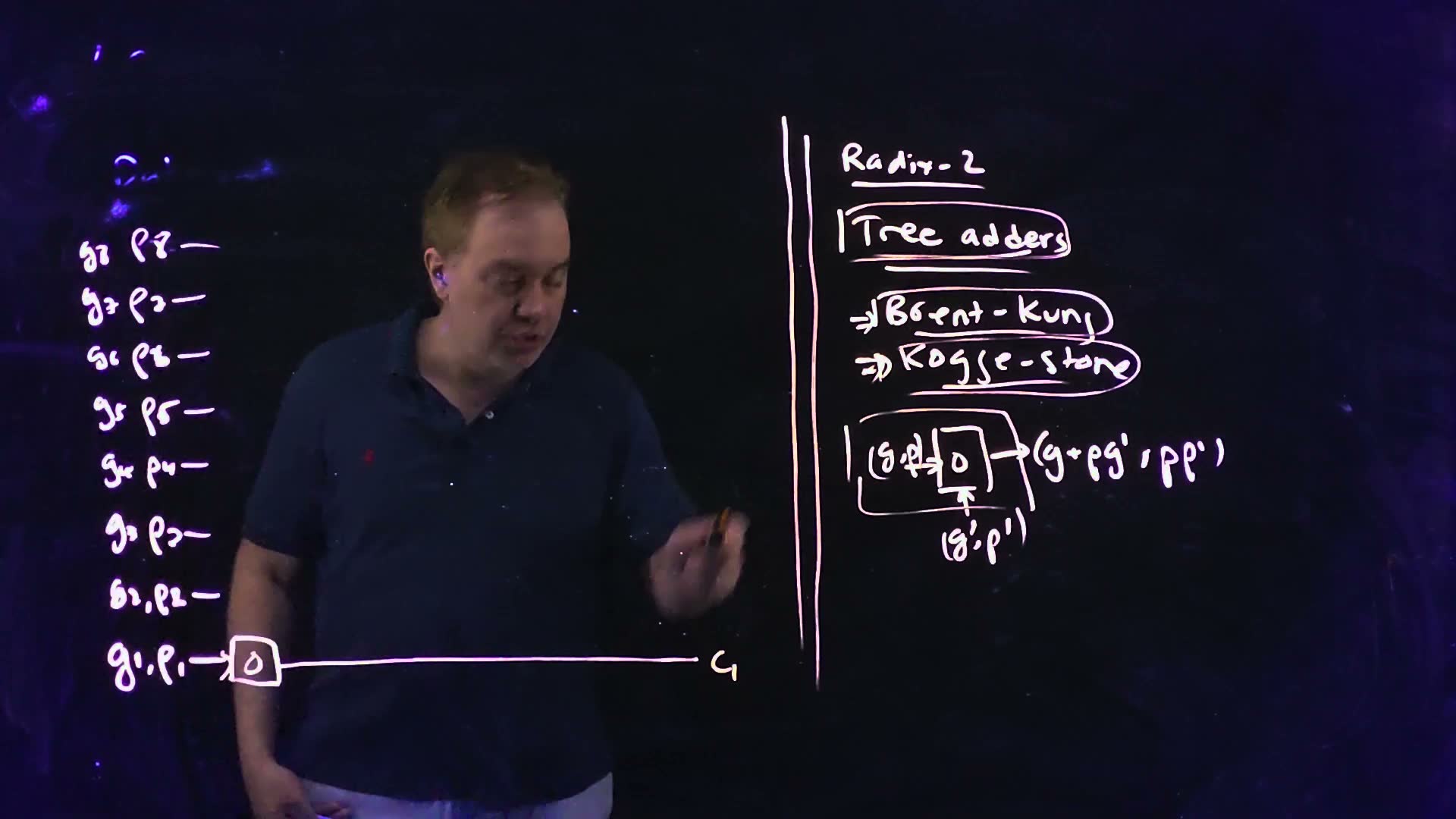
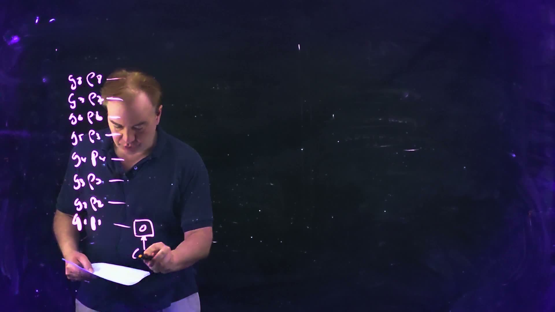
1. The inputs (03:53–04:46) board. Eight bits, numbered 1 to 8 from the bottom. Each enters the network as its $(g_k, p_k)$ from its PG cell. The carry-in enters at the bottom as the pair $(c_{in}, 0)$ (05:21): position 0.
2. The goal (04:55–05:21). Every carry, in parallel. The first is one element: $(g_1, p_1)\circ(c_{in}, 0) = (g_1 + p_1c_{in},\ 0)$p1​cin​, 0), “my carry, my C1, my carry out of my first bit position” (05:38). Its span is 1:0.
3. Every carry is a prefix added. In the same way, the carry out of bit $k$ is the group generate of everything from position 0 to bit $k$k: $C_k = G_{k:0}$Gk:0​. Each is a prefix of the row of positions, which is why these are called prefix adders; the lecture calls them radix-2 tree adders. Since position 0 has $p = 0$0, $P_{k:0} = 0$ for every $k$k: only the $G$ half of a carry span matters.
4. The sums added. Bit $k$ adds its own $p_k$ to the carry into it, which is the carry out of the bit below: $s_1 = p_1\oplus c_{in}$ and $s_k = p_k\oplus C_{k-1}$Ck−1​. In Chapter 16’s numbering, where bit $i$ there is bit $i + 1$ here, this is $s_i = p_i\oplus c_i$ci​; only the label moved.
5. The serial chain added. The simplest network makes the prefixes one after another: $C_1 = (g_1, p_1)\circ(c_{in}, 0)$(cin​,0), then $C_2 = (g_2, p_2)\circ C_1$C1​, and so on, $C_k = (g_k, p_k)\circ C_{k-1}$Ck−1​. Eight elements in a line, 8 levels to $C_8$C8​. Each element is Chapter 16’s carry stage, $c_{out} = g + p\,c_{in}$pcin​: this is the ripple-carry adder again.
6. How fast a tree could be added. By associativity, $G_{8:0}$ can be bracketed any way, for example $(G_{8:5}\circ G_{4:1})\circ(c_{in}, 0)$(cin​,0). But each element has only two inputs, so after one level a signal depends on at most 2 positions, after two on at most 4, after $L$ levels on at most $2^L$2L. $C_k$ depends on the $k + 1$ positions 0 to $k$k, so it needs at least $\lceil\log_2(k + 1)\rceil$ levels. For $C_8$C8​, nine positions: $2^3 = 8$ is too few, so at least 4 levels.

Every carry is a prefix added: $C_k = G_{k:0}$Gk:0​, the group generate from bit $k$ down to the carry-in at position 0. Made one element after another, $C_k = (g_k, p_k)\circ C_{k-1}$Ck−1​, each element adds one bit to the span: this is the ripple-carry adder, eight levels in series for eight bits.

Carries and sums of a prefix adderadded

$$\begin{gathered} C_k = G_{k:0},\qquad c_{out} = C_N\\ s_1 = p_1\oplus c_{in},\qquad s_k = p_k\oplus C_{k-1} \end{gathered}$$

Holds when: bits 1 … N with the carry-in at position 0 as (c_in, 0); the board writes C_k for the span 0–k (05:21)

The fastest any radix-2 network can beadded

$$\text{levels to } C_k \ \ge\ \lceil\log_2(k + 1)\rceil$$

Holds when: two-input elements; levels counted without fan-out

Memorize or derive. Memorize $C_k = G_{k:0}$ and $s_k = p_k\oplus C_{k-1}$Ck−1​: the sum takes the carry of the bit below. Derive the bound in two lines: an element at most doubles the number of positions a signal depends on, and $C_k$ depends on $k + 1$ of them.

A worked example added. $a = 0110$ (6), $b = 0011$ (3), $c_{in} = 0$0, through the serial chain.

bit $k$	4	3	2	1
$a_k$	0	1	1	0
$b_k$	0	0	1	1
$(g_k, p_k)$	(0, 0)	(0, 1)	(1, 0)	(0, 1)
$C_k$ (out of bit $k$k)	0	1	1	0
$s_k = p_k\oplus C_{k-1}$	1	0	0	1

$C_1 = g_1 + p_1c_{in} = 0 + 1\cdot0 = 0$0; $C_2 = g_2 + p_2C_1 = 1$ (bit 2 generates); $C_3 = 0 + 1\cdot1 = 1$ (bit 3 passes it); $C_4 = 0 + 0\cdot1 = 0$ (bit 4 kills it). Sums from bit 1 up: $s_1 = 1\oplus0 = 1$1, $s_2 = 0\oplus0 = 0$0, $s_3 = 1\oplus1 = 0$0, $s_4 = 0\oplus1 = 1$1. So $s = 1001 = 9$ with $c_{out} = C_4 = 0$0, and $6 + 3 = 9$9. §6 gets the same carries from a tree.

Traps.

• $s_k = p_k\oplus C_k$Ck​. $C_k$ is the carry out of bit $k$k; using it shifts every sum one place up. With $a_1 = b_1 = 1$ and $c_{in} = 0$ it gives $s_1 = 0\oplus1 = 1$1, but $1 + 1 = 10_2$ has $s_1 = 0$0.
• Leaving out the carry-in. A network over bits 1 to $N$ alone computes $G_{k:1}$Gk:1​, which are the carries only when $c_{in} = 0$0. Position 0 is what makes the adder take a carry in.

Check yourself Which two signals does s₅ need, and which span is its carry?

$p_5$ from bit 5’s PG cell and $C_4 = G_{4:0}$G4:0​, the carry out of bit 4: $s_5 = p_5\oplus G_{4:0}$G4:0​.

Check yourself Why can no network of radix-2 elements deliver C₈ in 3 levels, however it is wired?

Step 1: $C_8 = G_{8:0}$ depends on nine positions, $c_{in}$ and bits 1 to 8. Step 2: each element has two inputs, so after 3 levels a signal can depend on at most $2^3 = 8$ positions. Nine do not fit; 4 levels ($2^4 = 16$24=16) do.

3. The Kogge–Stone adder

You need

The element and its order (§1): $(G_{hi}, P_{hi})\circ(G_{lo}, P_{lo}) = (G_{hi} + P_{hi}G_{lo},\ P_{hi}P_{lo})$Phi​Glo​, Phi​Plo​), the higher span on the left, the lower from below; the spans must touch.

The radix-2 element (§1). Original figure ↑

What the network must produce (§2). The carry out of bit $k$ is the prefix $C_k = G_{k:0}$Gk:0​, with the carry-in entered as $(c_{in}, 0)$ at position 0. Any network needs at least $\lceil\log_2(k + 1)\rceil$ levels for $C_k$Ck​; the serial chain takes $k$k.

The serial chain (§2): one element per bit, 8 levels. Original figure ↑

The question. How can the eight carries be built so that every one of them arrives as early as the bound allows?

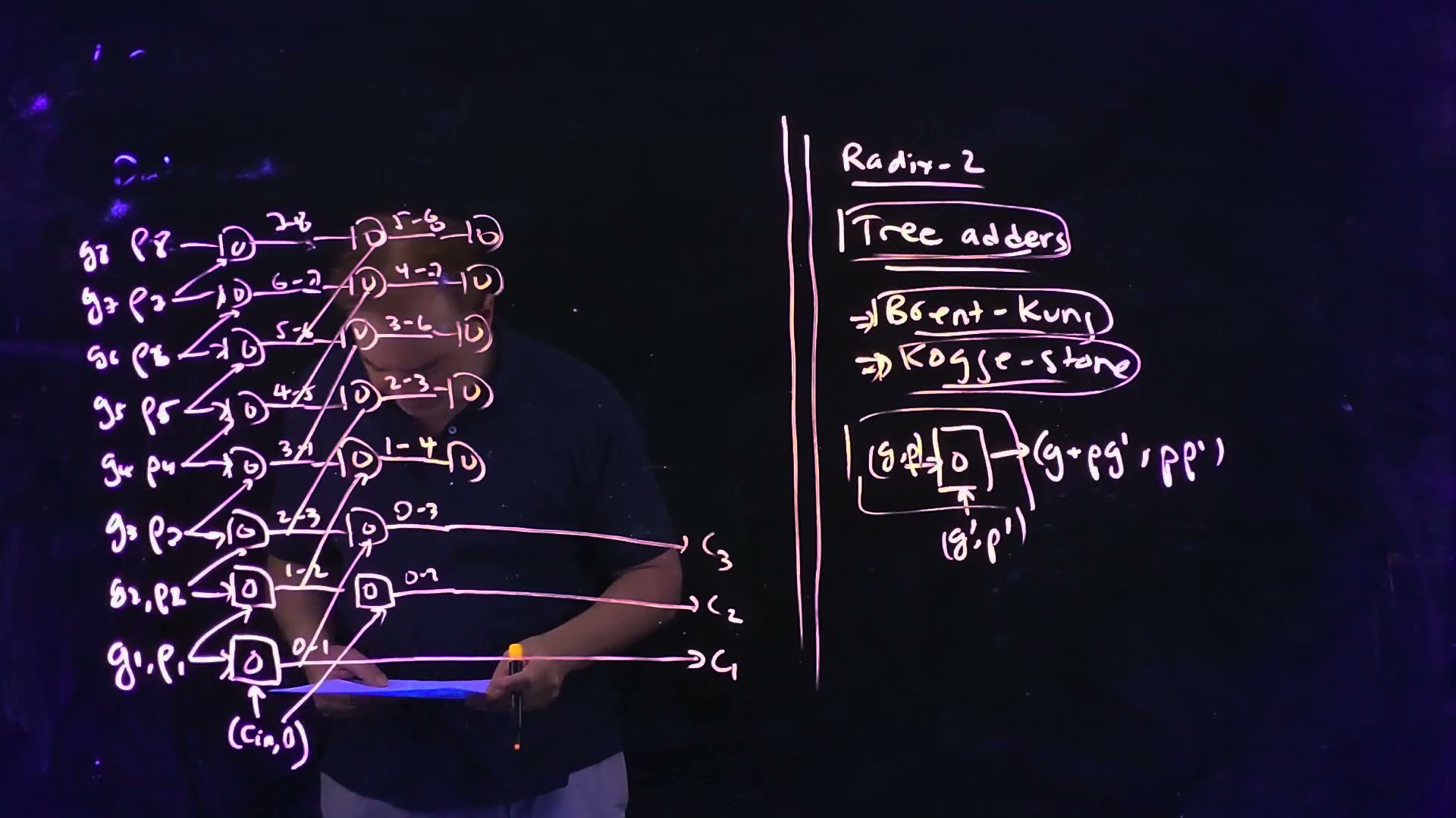
The idea is doubling. After one column of elements, each row holds a span of 2 positions; after the second, 4; after the third, 8. A row stops as soon as its span reaches position 0, because it then holds its carry. The board builds it column by column (05:21–09:58) board; the table lists every row’s span after each column.

Kogge–Stone, column by column (board, 05:21–09:58)

1. Column 1 (05:21–06:46). Every row merges with the row directly below it: 1:0 (bit 1 with $(c_{in}, 0)$(cin​,0), giving $C_1$C1​), then 2:1, 3:2, 4:3, 5:4, 6:5, 7:6, 8:7. Eight elements.
2. Column 2 (06:46–07:31). Each unfinished row merges with the row two below: 2:0 = 2:1 ∘ $(c_{in}, 0)$ gives $C_2$C2​; 3:0 = 3:2 ∘ 1:0 gives $C_3$C3​; then 4:1 = 4:3 ∘ 2:1, 5:2, 6:3, 7:4 and 8:5. Seven elements; rows 1 to 3 are done.
3. Column 3 (07:31–09:32). Each unfinished row merges with the row four below: 4:0 = 4:1 ∘ $(c_{in}, 0)$(cin​,0), 5:0 = 5:2 ∘ 1:0, 6:0 = 6:3 ∘ 2:0, 7:0 = 7:4 ∘ 3:0, and 8:1 = 8:5 ∘ 4:1. Five elements; rows 4 to 7 are done.
4. Column 4 (09:32–09:58). Row 8 merges with the row eight below: 8:0 = 8:1 ∘ $(c_{in}, 0)$ gives $C_8$C8​. One element. The rule: in column $m$m, every unfinished row merges with the row $2^{m-1}$ below it.
5. What the lecturer likes about it (09:58–11:47). “This is Kogge–Stone. Has this particular pattern, this particular regularity” (10:28). Every element’s output drives one or two other elements (the last carries, 4:0 to 8:0, drive none), so “very relatively consistent fan out, which means that the sizing of these blocks can be … much more uniform” (11:38): one element design serves everywhere. The one exception is not an element: the carry-in entry, a primary input, drives four, 1:0, 2:0, 4:0 and 8:0, which is why the board writes $(c_{in}, 0)$ twice.
6. How deep each carry is added. $C_1$ is 1 level deep, $C_2$ and $C_3$ are 2, $C_4$ to $C_7$ are 3, and $C_8$ is 4: every carry meets its bound $\lceil\log_2(k + 1)\rceil$ from §2. No radix-2 network does better.

row $k$	after column 1	column 2	column 3	column 4	depth of $C_k$
8	8:7	8:5	8:1	8:0	4
7	7:6	7:4	7:0		3
6	6:5	6:3	6:0		3
5	5:4	5:2	5:0		3
4	4:3	4:1	4:0		3
3	3:2	3:0			2
2	2:1	2:0			2
1	1:0				1

The Kogge–Stone network as the board builds it (Lecture16 @ 10:41), redrawn. Each row is a bit position, bit 1 at the bottom; the carry-in enters once, as the pair $(c_{in}, 0)$ in row 0 at the bottom, where the board writes it twice. Each element takes its higher input along its own row from the left and its lower input on a diagonal from a lower row; the label above each output is its span, high index first (the board writes 0–8 for 8:0). Column $m$ (grey numbers, added) combines spans $2^{m-1}$ rows apart. Row $k$ ends in the carry $C_k = G_{k:0}$Gk:0​. 21 elements, 4 levels.

The board (Lecture16 @ 10:41)

Lecture16 @ 10:41The Kogge–Stone network: 21 elements in four columns, carries C₁ to C₈ at the right.

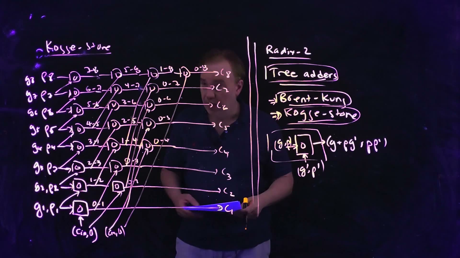
Fair copy of the board above (Lecture16 @ 10:41), mark for mark in its own layout. All black: one cream pen wrote the network, and the right half is 03:32’s, with “Tree adders” now boxed. The three small strokes at the top left are what is left of the wiped recap. Span labels are copied as the board writes them, low index first (“7–8” is the span 8:7); where a diagonal crosses a label, the label sits on a white patch. The lecturer’s 7 looks like a 2 throughout (in “7–8”, “6–7”, $C_7$ and $g_7\,p_7$g7​p7​), and the title’s gg look like ss; they are set as 7 and “Kogge”. The lower input of the 8:5 element carries its arrowhead at its row-6 end, as drawn.

The cone of $C_8$ added: the Kogge–Stone network (Lecture16 @ 10:41, redrawn) with the eight elements that build $C_8 = G_{8:0}$ drawn thick: 8:7, 6:5, 4:3 and 2:1 in column 1, 8:5 and 4:1 in column 2, 8:1 in column 3 and 8:0 in column 4. They form a balanced binary tree over the nine inputs, so $C_8$ is four levels deep.

Kogge–Stone countsadded

$$\text{levels} = \lceil\log_2(N + 1)\rceil,\qquad \text{elements in column } m = N + 1 - 2^{m-1}$$

Holds when: N bits with the carry-in, so N + 1 positions; column m merges rows 2^(m−1) apart and stops a row once it reaches position 0

Memorize or derive. Memorize the rule (column $m$ reaches $2^{m-1}$ rows down). Derive the counts: in column $m$ the rows $0$ to $2^{m-1} - 1$ are already finished, so the other $N + 1 - 2^{m-1}$ rows each get an element. For 8 bits that is $8 + 7 + 5 + 1 = 21$21.

A worked example added. The board’s network has 21 elements in 4 levels, with carry depths 1, 2, 2, 3, 3, 3, 3, 4 for $C_1$ to $C_8$C8​. A 16-bit Kogge–Stone with a carry-in has 17 positions: $\lceil\log_2 17\rceil = 5$ levels and $16 + 15 + 13 + 9 + 1 = 54$ elements. Check: the cone of $C_8$ in the figure is a balanced tree over nine leaves, eight elements and four levels deep, which is the bound for nine positions.

Traps.

• Merging with the row directly below in every column. That is the serial chain again: each column then adds only one position.
• Reading the board’s top label “2–8” as a span from 2. It is 7–8 (the lecturer’s 7 has a crossbar and curl); the element sits in column 1 of row 8, so it can only be 8:7.

Check yourself Which two spans make 6:0 in the Kogge–Stone network, and in which column?

6:3 (row 6 after column 2) and 2:0 (row 2’s finished carry, four rows below): $G_{6:0} = G_{6:3} + P_{6:3}G_{2:0}$P6:3​G2:0​, in column 3.

Check yourself In a 16-bit Kogge–Stone with a carry-in, at which level does C₁₁ arrive, and which two spans make it?

Step 1: $C_{11}$ covers 12 positions, so it needs $\lceil\log_2 12\rceil = 4$ levels, and Kogge–Stone meets the bound. Step 2: after three columns row 11 holds 11:4 (eight positions); column 4 merges it with the row eight below, row 3, which holds 3:0: $G_{11:0} = G_{11:4}\circ G_{3:0}$G3:0​.

4. The Brent–Kung adder

You need

The element and the target (§1, §2). Two touching spans merge, the higher on the left: $(G_{hi} + P_{hi}G_{lo},\ P_{hi}P_{lo})$Phi​Glo​, Phi​Plo​). The network must produce every carry $C_k = G_{k:0}$Gk:0​, with the carry-in as $(c_{in}, 0)$ at position 0, and $C_8$ needs at least 4 levels.

The Kogge–Stone network (§3). Column $m$ merges each unfinished row with the row $2^{m-1}$ below: 21 elements, 4 levels, every carry as early as possible.

The Kogge–Stone network (§3; Lecture16 @ 10:41, redrawn): 21 elements. Original figure ↑

The question. Kogge–Stone spends 21 elements on 8 carries. Many of its spans, such as 5:2 or 6:3, are used once and thrown away. Can a network reuse a few spans and get by with far fewer elements?

The idea is to build power-of-two spans from position 0 (2:0, 4:0, then 8:0) and fill in the other carries from them. The lecturer motivates it before drawing it: “I’ll have many, many fewer of these look-ahead blocks in the Brent–Kung than I have in the Kogge–Stone” (11:56).

Brent–Kung on the same eight bits (board, 13:24–16:51)

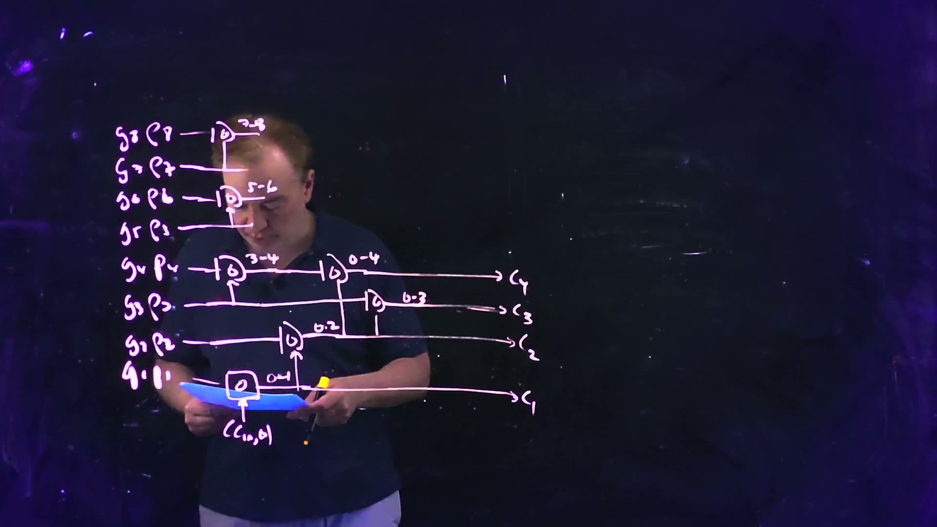
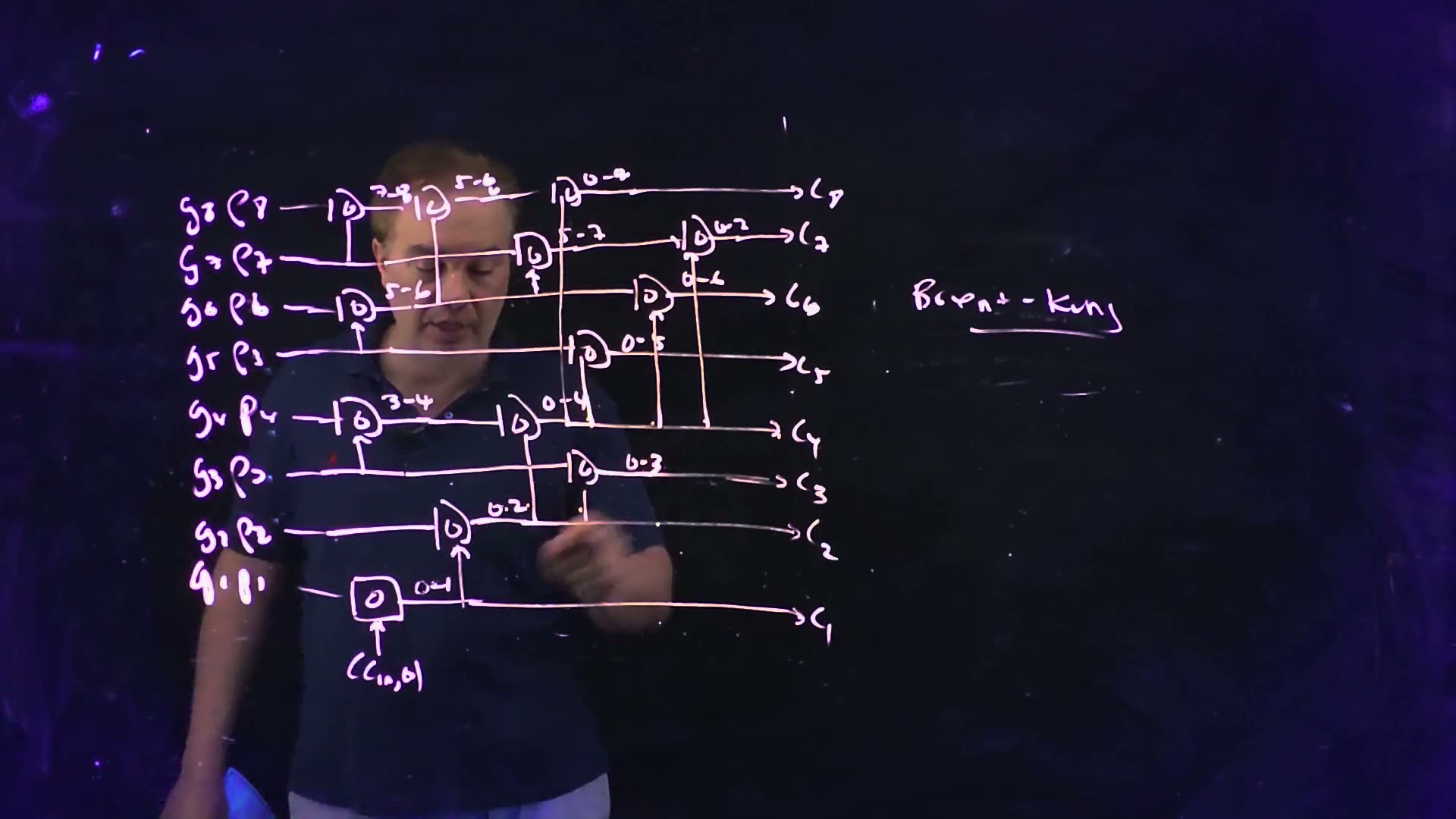
1. Pairs (13:24–14:19) board. 1:0 = bit 1 ∘ $(c_{in}, 0)$(cin​,0), which is already $C_1$C1​. Then the pairs 4:3, 6:5 and 8:7. Bit 2 is not paired: it joins 1:0 directly in the next step.
2. Powers of two from 0 (14:21–14:52) board. 2:0 = bit 2 ∘ 1:0 gives $C_2$C2​; 4:0 = 4:3 ∘ 2:0 gives $C_4$C4​.
3. Fill in (14:52–16:51) board. 3:0 = bit 3 ∘ 2:0 ($C_3$C3​); 5:0 = bit 5 ∘ 4:0; 6:0 = 6:5 ∘ 4:0; 7:5 = bit 7 ∘ 6:5, then 7:0 = 7:5 ∘ 4:0; 8:5 = 8:7 ∘ 6:5, then 8:0 = 8:5 ∘ 4:0. Each lower input rises on a vertical wire from a lower row. Thirteen elements.
4. The price: fan-out (14:59–15:26, 17:02–17:29). The reused spans drive many loads. “The fan out here is very irregular, right? Look at this guy here. It fans out here, here, here, here, and here” (17:19): the 4:0 node drives 5:0, 6:0, 7:0, 8:0 and the $C_4$ output, five loads. The 2:0 node drives three (3:0, 4:0 and $C_2$C2​), and so does the 6:5 node (6:0, 7:5 and 8:5).
5. How deep each carry is added. $C_1$ 1 level, $C_2$ 2, $C_3$ and $C_4$ 3, $C_5$ to $C_8$ 4. $C_8$ arrives at level 4, as in Kogge–Stone, but $C_3$ and $C_5$ to $C_7$ are a level later than their bound.
6. The board’s variant added. The strict Brent–Kung pattern would make 7:0 as bit 7 ∘ 6:0: one element fewer (12), but 6:0 is already 4 levels deep, so 7:0 would be 5. The board spends the extra element 7:5 to keep every carry within 4 levels. This chapter teaches the board’s network; §5’s general counts use the strict pattern.

The Brent–Kung network as the board builds it (Lecture16 @ 17:54; $C_1$C1​, behind the lecturer’s hands there, from 17:26), redrawn. The rows and inputs are those of the Kogge–Stone figure, with the carry-in drawn once in row 0; each lower input rises on a vertical wire from a lower row. Pairs (4:3, 6:5, 8:7) and the chain 1:0, 2:0, 4:0 go up; 4:0 then serves 5:0, 6:0, 7:0 and 8:0. Spans are written high index first (the board writes 0–8 for 8:0). 13 elements, 4 levels.

The board (Lecture16 @ 17:54)

Lecture16 @ 17:54The Brent–Kung network: 13 elements; the 0–4 node feeds four elements and C₄.

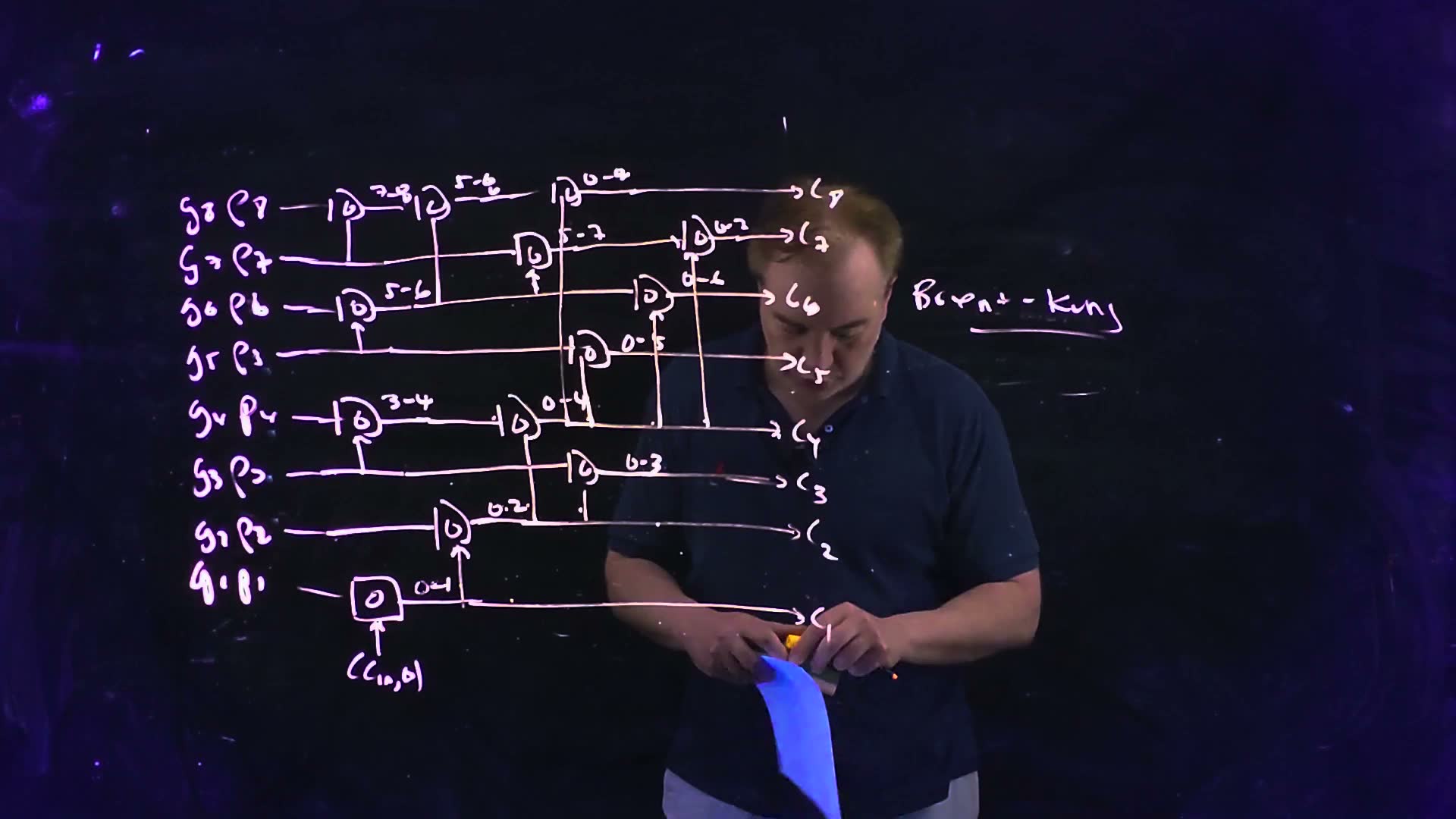
Fair copy of the board above (Lecture16 @ 17:54), mark for mark in its own layout. All black: one cream pen wrote the board; the small strokes at the top left and top middle are left from the wiped boards. $C_1$ and the end of its wire, under the lecturer’s hands here, are copied from 17:26. Span labels are copied as the board writes them, low index first (“0–4” is the span 4:0). The lecturer’s 7 looks like a 2 (in “0–7”), his 8 like a 6 over an o (in “5–8”) or a 9 (in $C_8$C8​), and the g of “Kung” like a y; they are set as what they are. The lower input of the 3:0 element is a short stroke that stops below the element, as drawn.

Fan-out in the Brent–Kung network added (Lecture16 @ 17:54, redrawn). The 4:0 node (thickest) drives four elements, 5:0, 6:0, 7:0 and 8:0, and the output $C_4$C4​: a fan-out of 5. The 2:0 node (3:0, 4:0 and $C_2$C2​) and the 6:5 node (6:0, 7:5 and 8:5) drive three each (medium). Kogge–Stone’s element outputs drive at most three, counting a carry output (its carry-in entry, a primary input, drives four).

Memorize or derive. Memorize the shape: pair up, build 2:0, 4:0, 8:0 from position 0, then fill in. Derive the element count and each carry’s depth by drawing it; there is no new formula here.

A worked example added. Counted on the board’s network: 13 elements against Kogge–Stone’s 21; carry depths 1, 2, 3, 3, 4, 4, 4, 4 against 1, 2, 2, 3, 3, 3, 3, 4; the largest fan-out of an element output 5 against 3 (Kogge–Stone’s carry-in entry, a primary input, drives four). Check: add one element per new carry and per pair: the four pair elements (1:0, 4:3, 6:5, 8:7), the seven other carries (2:0 to 8:0) and the two helpers 7:5 and 8:5 make $4 + 7 + 2 = 13$13.

Traps.

• “Fewer elements, so fewer levels.” The elements saved are the parallel ones. The chain through 4:0 gets longer, and the 4:0 node is heavily loaded.
• Pairing bit 2 with bit 1. On the board 1:0 already contains $c_{in}$cin​; bit 2 joins it directly as 2:0, and the pairs start at 4:3.

Check yourself Which two spans make 6:0 in the Brent–Kung network?

6:5 (the pair of bits 6 and 5) and 4:0: $G_{6:0} = G_{6:5} + P_{6:5}G_{4:0}$P6:5​G4:0​.

Check yourself Suppose the 4:0 node is slow because of its load. Which carries wait for it, and which sums does that delay?

Step 1: $C_4$ is the node itself, and 5:0, 6:0, 7:0 and 8:0 all take it as their lower input: $C_4$ to $C_8$ wait. Step 2: the sums that use them are $s_5$ to $s_8$ (each $s_k$ takes $C_{k-1}$Ck−1​), and $c_{out} = C_8$C8​. Only $s_1$ to $s_4$ are unaffected.

5. Kogge–Stone against Brent–Kung: levels, elements, fan-out

You need

The two networks (§3, §4). Kogge–Stone merges each row with the row $2^{m-1}$ below in column $m$m: 21 elements for 8 bits, every carry at its bound. Brent–Kung pairs up, builds 2:0, 4:0, 8:0 and fills in: 13 elements, but several carries a level later, and the 4:0 node drives five loads.

Kogge–Stone (§3): 21 elements, 4 levels. Original figure ↑

Brent–Kung (§4): 13 elements, 4 levels. Original figure ↑

Load and sizing (Chapter 8, §1). A gate’s delay grows with the capacitance it drives, its electrical effort $h$h, unless the gate is made larger. A node with many loads is slow or needs a bigger driver; a design in which every node has about the same load can use one size everywhere.

The question. Both 8-bit networks deliver $C_8$ in 4 levels. Which is faster, which is smaller, and how does the difference grow with the width?

The comparison (spoken 11:07–12:22 and 17:02–17:40; numbers added)

1. What the lecturer says (11:07–12:22, 17:02–17:40). Kogge–Stone is regular, and every element’s output drives “either two or one” others, so the elements can be sized uniformly (11:38). Brent–Kung has “many, many fewer” elements (11:56), is “much more area efficient” (12:04) and takes “much less area” (17:38), but its fan-out is very irregular, so its elements need several sizes. Every advantage he gives Brent–Kung is about area.
2. Each carry’s depth added. Kogge–Stone 1, 2, 2, 3, 3, 3, 3, 4; Brent–Kung 1, 2, 3, 3, 4, 4, 4, 4. The sum $s_k$ needs $C_{k-1}$Ck−1​, so $s_4$s4​, $s_6$s6​, $s_7$ and $s_8$ wait one level longer in Brent–Kung (they need $C_3$C3​, $C_5$C5​, $C_6$ and $C_7$C7​). $s_5$ does not: $C_4$ is at level 3 in both.
3. Example delays added. With the PG cell’s delay $t_{PG} = 2$2, one element’s $t_e = 4$ and the sum XOR’s $t_{sum} = 4\,\tau_{inv}$ (for example; $\tau_{inv}$ is the fan-out-of-one inverter delay), the top sum $s_8$ is ready at $t_{PG} + 3t_e + t_{sum} = 18\,\tau_{inv}$ in Kogge–Stone ($C_7$C7​ at level 3) and at $t_{PG} + 4t_e + t_{sum} = 22\,\tau_{inv}$ in Brent–Kung ($C_7$C7​ at level 4). $c_{out} = C_8$ is at $t_{PG} + 4t_e = 18\,\tau_{inv}$ in both. The serial chain of §2 reaches $s_8$ at $t_{PG} + 7t_e + t_{sum} = 34\,\tau_{inv}$34τinv​: Chapter 16’s ripple count, $(N - 1)t_c + t_{sum} = 32$32, plus the PG cell in front.
4. Growth with the width added. For $N$ positions, $N$ a power of 2, Kogge–Stone takes $\log_2 N$ levels and $N\log_2 N - N + 1$ elements; the strict Brent–Kung pattern takes $2\log_2 N - 2$ levels and $2N - 2 - \log_2 N$ elements. At 64 positions that is 6 levels against 10, and 321 elements against 120.
5. Wiring added. Kogge–Stone’s other cost is its wires. On the 8-bit board, column $m$ runs $9 - 2^{m-1}$ lower-input wires, each $2^{m-1}$ rows long: the board’s long diagonals. Summed per lower input, the lower-input wires span 50 row pitches in Kogge–Stone and 21 in Brent–Kung. Brent–Kung shares some verticals (4:0’s single wire up to 8:0 feeds four elements), so its true wiring is shorter still.
6. The verdict. Kogge–Stone is the faster adder: every carry at the bound, low and even fan-out. Brent–Kung is the smaller one: fewer elements, less area, fewer long wires, but more levels for half the carries at 8 bits ($C_3$C3​, $C_5$C5​, $C_6$C6​, $C_7$C7​) and for most of them from 32 positions on, and loaded nodes.

The level at which each carry $C_k$ is ready added, computed from the two board networks (Lecture16 @ 10:41 and 17:54). Kogge–Stone (solid) reaches every carry at the lower bound $\lceil\log_2(k+1)\rceil$1)⌉; Brent–Kung (hatched) matches it at $C_1$C1​, $C_2$C2​, $C_4$ and $C_8$ but delivers $C_3$ and $C_5$–$C_7$ one level later, so the sums $s_4$ and $s_6$–$s_8$ wait longer.

Levels (left) and elements (right) against the number of positions $N$ added, computed from the general constructions ($N$N a power of 2): Kogge–Stone needs $\log_2 N$ levels and $N\log_2 N - N + 1$ elements; the strict Brent–Kung pattern needs $2\log_2 N - 2$ levels and $2N - 2 - \log_2 N$ elements. Brent–Kung’s levels grow twice as fast; at 64 positions it has 120 elements against 321.

$N$ positions	4	8	16	32	64
KS levels	2	3	4	5	6
KS elements	5	17	49	129	321
BK levels	2	4	6	8	10
BK elements	4	11	26	57	120

The board’s 8-bit adders have 9 positions (with $c_{in}$cin​), so they fall between the table’s 8 and 16 columns: 21 and 13 elements, 4 levels each (§3, §4).

Prefix network countsadded

$$\begin{aligned} \text{KS:}&\quad \log_2 N \text{ levels},\quad N\log_2 N - N + 1 \text{ elements}\\ \text{BK:}&\quad 2\log_2 N - 2 \text{ levels},\quad 2N - 2 - \log_2 N \text{ elements} \end{aligned}$$

Holds when: N positions, N a power of 2 (with a carry-in, N − 1 bits); levels counted without fan-out; Brent–Kung in its strict pattern (the board's 8-bit variant has 13 elements and 4 levels)

Memorize or derive. Memorize the verdict: Kogge–Stone fast and regular but large, Brent–Kung small but deeper and irregular. Derive the counts when needed. Kogge–Stone: $\log_2 N$ columns, and column $m$ has $N - 2^{m-1}$ elements, so the total is $N\log_2 N - (N - 1)$1). Brent–Kung: the up-sweep builds the power-of-two spans in $\log_2 N$ levels with $N - 1$ elements; the down-sweep fills in the other carries in $\log_2 N - 2$ more levels with $N - 1 - \log_2 N$ elements.

A worked example added. Take $N = 16$ positions. Kogge–Stone: four columns, combining rows 1, 2, 4 and 8 apart, of $16 - 1$1, $16 - 2$2, $16 - 4$ and $16 - 8$ elements: $15 + 14 + 12 + 8 = 49$ elements in 4 levels. Brent–Kung: the up-sweep builds the power-of-two spans with $8 + 4 + 2 + 1 = 15$ elements in 4 levels and makes four of the 15 carries (1:0, 3:0, 7:0, 15:0); the down-sweep adds one element for each of the other $15 - 4 = 11$11, the last of them (14:0) at level 6. So 26 elements and 6 levels. Check: the formulas give $16 \times 4 - 16 + 1 = 49$ and $2 \times 16 - 2 - 4 = 26$ elements, $\log_2 16 = 4$ and $2 \times 4 - 2 = 6$ levels, as in the table; the gap of 2 levels is $\log_2 N - 2$2, which is 0 at $N = 4$ and opens from $N = 8$8.

Traps.

• “Brent–Kung is faster.” The lecturer once says so (12:45), right after listing its area savings; the boards and the counts say otherwise. Brent–Kung is the smaller adder, never the faster one.
• Comparing only $c_{out}$cout​. In the 8-bit networks both put $C_8$ at level 4; the difference is in the carries the sums need.

Check yourself At 32 positions, how many more elements does Kogge–Stone use than Brent–Kung?

$129 - 57 = 72$72: Kogge–Stone $32 \times 5 - 32 + 1 = 129$129, Brent–Kung $2 \times 32 - 2 - 5 = 57$57.

Check yourself For a 64-position adder with the example element delay t_e = 4 τ_inv, how much sooner is Kogge–Stone's last carry than Brent–Kung's, counting levels only?

Step 1: levels: Kogge–Stone $\log_2 64 = 6$6, Brent–Kung $2 \times 6 - 2 = 10$10. Step 2: $(10 - 6) \times 4 = 16\,\tau_{inv}$ sooner. The PG cell and the sum XOR are the same in both, so they cancel.

6. The whole prefix adder: PG, network, sums

You need

The PG cell and the sum (Chapter 16, §9). Each bit’s PG cell makes $g_k = a_kb_k$ and $p_k = a_k\oplus b_k$bk​; the sum is $p_k$ XOR the carry into the bit. The propagate must be the XOR, not $a + b$b, because the sum reuses it.

Chapter 16’s PG cell, and the carry and sum from $g$ and $p$ (§9). Original figure ↗

The carries (§2). $C_k = G_{k:0}$ is the carry out of bit $k$k, with the carry-in as $(c_{in}, 0)$ at position 0; so $s_1 = p_1\oplus c_{in}$ and $s_k = p_k\oplus C_{k-1}$Ck−1​.

A network (§3). Kogge–Stone: in column $m$ each unfinished row merges with the row $2^{m-1}$ below.

The 8-bit Kogge–Stone network (§3). Original figure ↑

The question. FN17-8 asks for the complete adder, not only the network. How do the PG cells, the network and the sum XORs connect, and where is the critical path?

The lecture draws only the networks. The assembly is added here added, at 4 bits so that every wire can be checked by hand. It is drawn as FN17-8’s paper draws its adder: the highest bit at the left, so the carry-in comes in from the right.

A 4-bit Kogge–Stone adder (added)

1. Three rows of blocks. At the bottom, one PG cell per bit. In the middle, the network over positions 0 to 4. At the top, one sum XOR per bit. $(c_{in}, 0)$ enters the network at position 0.
2. The network. Kogge–Stone over five positions: level 1 makes 1:0, 2:1, 3:2 and 4:3; level 2 makes 2:0 (2:1 ∘ $c_{in}$cin​), 3:0 (3:2 ∘ 1:0) and 4:1 (4:3 ∘ 2:1); level 3 makes 4:0 (4:1 ∘ $c_{in}$cin​). Eight elements, 3 levels.
3. The sums. $s_1 = p_1\oplus c_{in}$cin​, $s_2 = p_2\oplus C_1$C1​, $s_3 = p_3\oplus C_2$C2​, $s_4 = p_4\oplus C_3$C3​, and $c_{out} = C_4$C4​. Each sum takes its $p_k$ on a wire straight up from its own PG cell, past the network, and its carry from the column of the bit below it, which in this drawing is the column to its right.
4. The critical path. Trace each output back to the inputs. $s_4$ needs $C_3 = G_{3:0}$G3:0​, which is 2 levels deep: $a_3, b_3$ → PG → 3:2 → 3:0 → $s_4$s4​, so $t_{PG} + 2t_e + t_{sum}$ (the delays of the PG cell, one element and the sum XOR, §5). $c_{out}$ needs $C_4$C4​, 3 levels deep: $a_4, b_4$ → PG → 4:3 → 4:1 → 4:0, so $t_{PG} + 3t_e$3te​. With the example values both are $14\,\tau_{inv}$14τinv​. Which one is “the” critical path depends on the sum XOR against one element: if $t_{sum} > t_e$ the top sum is, otherwise $c_{out}$ is. On the exam, mark both and say why.

A 4-bit prefix adder added, drawn with bit 4 at the left as FN17-8’s paper draws its adder. Bottom: the PG cells give $g_k, p_k$gk​,pk​. Middle: a 4-bit Kogge–Stone network in three levels (grey numbers); each element takes its higher input from below and its lower input from the right, and the carry-in enters at the right as $(c_{in}, 0)$(cin​,0). Top: each sum XOR forms $s_k = p_k\oplus C_{k-1}$Ck−1​, so it takes its carry from the column to its right ($s_1$s1​ takes $c_{in}$cin​). Thick: the path to the top sum, through bit 3’s PG cell, 3:2 and 3:0 (two levels). Thick dashed: the path to $c_{out}$cout​, through 4:3, 4:1 and 4:0 (three levels).

The prefix adder's critical pathadded

$$t_{s_N} \approx t_{PG} + L\,t_e + t_{sum},\qquad t_{c_{out}} \approx t_{PG} + L'\,t_e$$

Holds when: L = the depth of C_(N−1), the carry the top sum needs; L′ = the depth of C_N; delays counted per element, fan-out ignored

Memorize or derive. Derive by tracing: PG, then the levels of the carry the output needs, then the sum (or nothing, for $c_{out}$cout​). Remember only that the top sum needs $C_{N-1}$CN−1​, not $C_N$CN​.

A worked example added. §2’s addition, now through the tree: $a = 0110$0110, $b = 0011$0011, $c_{in} = 0$0, so bits 1 to 4 have $(g, p) = (0, 1)$(0,1), $(1, 0)$(1,0), $(0, 1)$(0,1), $(0, 0)$(0,0).

level	span	inputs (higher ∘ lower)	$(G, P)$
1	1:0	$(0, 1)\circ(0, 0)$	(0, 0)
1	2:1	$(1, 0)\circ(0, 1)$	(1, 0)
1	3:2	$(0, 1)\circ(1, 0)$	(1, 0)
1	4:3	$(0, 0)\circ(0, 1)$	(0, 0)
2	2:0	2:1 ∘ $(c_{in}, 0)$ = $(1, 0)\circ(0, 0)$	(1, 0)
2	3:0	3:2 ∘ 1:0 = $(1, 0)\circ(0, 0)$	(1, 0)
2	4:1	4:3 ∘ 2:1 = $(0, 0)\circ(1, 0)$	(0, 0)
3	4:0	4:1 ∘ $(c_{in}, 0)$ = $(0, 0)\circ(0, 0)$	(0, 0)

The carries are the $G$ of the spans ending at 0: $C_1 \dots C_4 = 0, 1, 1, 0$0,1,1,0. The sums: $s_1 = 1\oplus0 = 1$1, $s_2 = 0\oplus0 = 0$0, $s_3 = 1\oplus1 = 0$0, $s_4 = 0\oplus1 = 1$1, so $s = 1001 = 9$ and $c_{out} = 0$0. Check: the serial chain of §2 gave the same carries, 0, 1, 1, 0, one bit at a time; and $6 + 3 = 9$9. Note 4:1: bit 4 kills the carry that bit 2 makes, so the span from 1 to 4 neither generates nor propagates.

Traps.

• $s_k = p_k\oplus C_k$Ck​, the sums one position too high. It is the commonest slip in drawing this adder: wiring each sum to the carry span of its own column, $G_{k:0}$Gk:0​, instead of the one below, $G_{k-1:0}$Gk−1:0​. With $a_1 = b_1 = 1$ and $c_{in} = 0$ it gives $s_1 = 0\oplus1 = 1$1, but $1 + 1 = 10_2$102​. In a 4-bit adder this wiring gets 350 of the 512 possible additions wrong.
• Feeding the sums from the network’s $P$ outputs. The sums need each bit’s own $p_k$pk​, straight from its PG cell, and only the $G$ of the carry span.

Check yourself Which block does C₄ feed in the 4-bit adder?

No sum: it is the carry out, $c_{out} = C_4$C4​. The top sum $s_4$ takes $C_3$C3​.

Check yourself In the board's 8-bit Kogge–Stone adder, which sums are the last to have their carries, and at what level? With the example delays, when is s₈ ready?

Step 1: $s_5$ to $s_8$ take $C_4$ to $C_7$C7​, which arrive at level 3 (and $s_4$s4​, $s_3$ take $C_3$C3​, $C_2$ at level 2). Step 2: $s_8$ is ready at $t_{PG} + 3t_e + t_{sum} = 2 + 12 + 4 = 18\,\tau_{inv}$18τinv​, the same time as $c_{out}$ ($2 + 4 \times 4 = 18$2+18).

7. Shifters: logical, arithmetic, rotator

You need

Two’s complement (Chapter 15, §11). In an $n$-bit two’s-complement word the MSB carries the weight $-2^{n-1}$−2n−1, so a word with MSB 1 is negative. To negate, invert every bit and add 1: $4 = 0000\,0100$00000100, so $-4 = 1111\,1011 + 1 = 1111\,1100$11111100.

Place value added. Moving every bit one place toward the MSB doubles an unsigned number ($0110 = 6$0110= becomes $1100 = 12$12); moving every bit one place toward the LSB halves it and drops the old LSB.

The question. A shifter slides a word’s bits left or right by some number of places. The bits that fall off one end are lost or reused, and the open end must be filled with something. What fills it, and why does the answer depend on what the word means?

Three kinds of shift (board, 17:40–22:47)

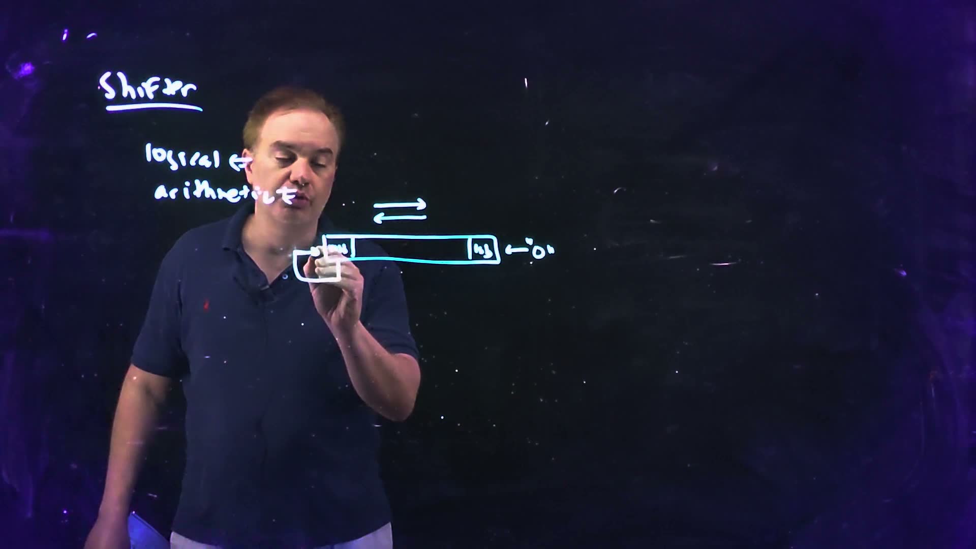
1. Logical (18:40–19:51) board. Shift either way and fill the open end with 0. The word is treated as a pattern of bits.
2. Arithmetic (19:51–21:37) board. A left shift fills with 0 and multiplies by 2 (“shift by 1”, $\times 2$ on the board). A right shift must divide by 2 and keep the sign: “If I divide minus four, I want to get minus two” (21:07). So the right shift fills the open MSB end with a copy of the MSB, sign extension: $-4 = 1111\,1100$ becomes $1111\,1110 = -2$−2, while a logical shift would give $0111\,1110 = 126$126.
3. Rotator (21:37–22:33) board. The bit that falls off one end comes back in at the other; nothing is lost. “Very commonly used in signal processing applications.”
4. One word, three ways added. Shift $1011\,0110$ ($-74$−74 in two’s complement; 182 unsigned) right by 2. Logical: $0010\,1101 = 45$45, a positive number. Arithmetic: $1110\,1101 = -19$−19. Rotate: $1010\,1101$10101101, the two dropped bits 10 now at the top.
5. Rounding added. An arithmetic right shift by $n$ gives $\lfloor x/2^n\rfloor$⌊x/2n⌋, rounding down. For $-74$ by 2: $-74/4 = -18.5$−18.5, and $\lfloor -18.5\rfloor = -19$−19, which is the arithmetic result. Rounding toward zero would give $-18$−18.

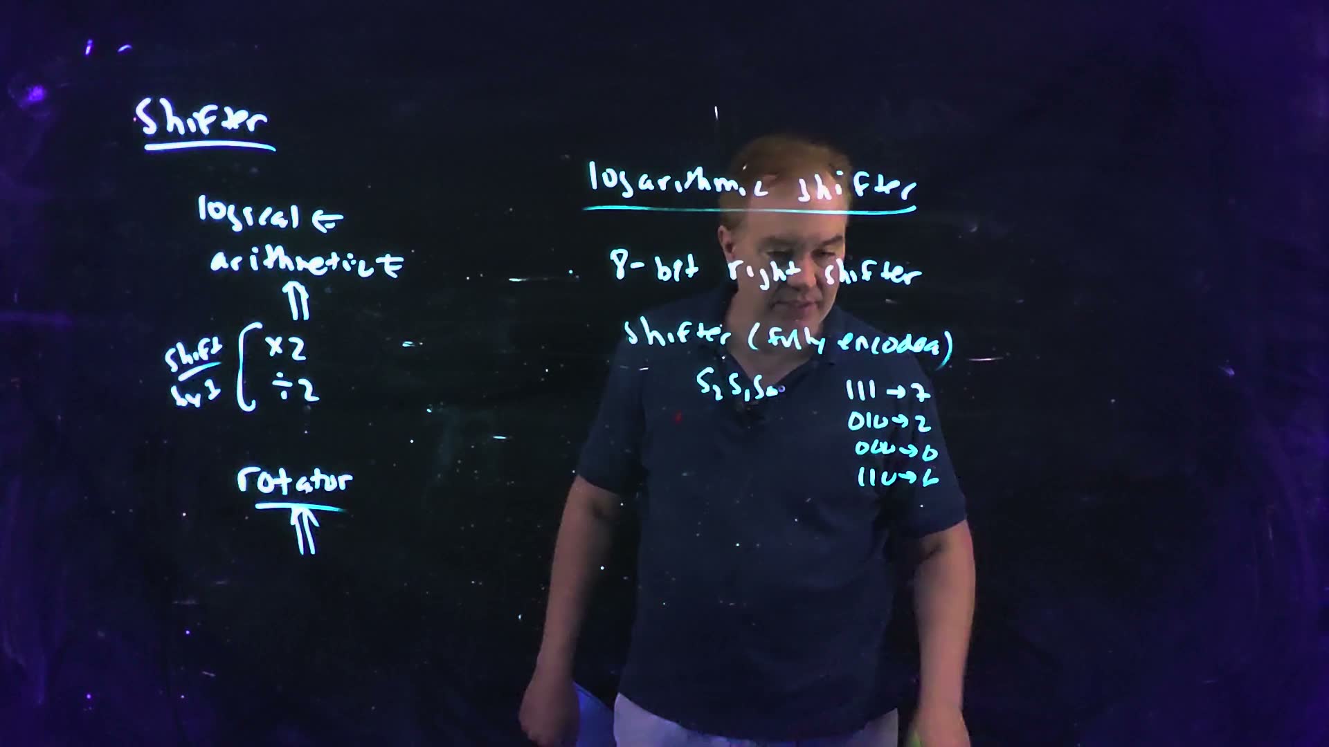
The three kinds of shift, redrawn from the board (Lecture16 @ 22:11), top to bottom. Logical: the word moves left or right and a 0 enters the end being vacated. Arithmetic: a left shift (×2) brings a 0 into the LSB; a right shift (÷2) copies the MSB back into itself, so the sign is kept (sign extension). Rotator: the bit leaving one end enters the other, in either direction.

The board (Lecture16 @ 22:11)

Lecture16 @ 22:11Shifters: logical and arithmetic (×2, ÷2, sign extension) and the rotator.

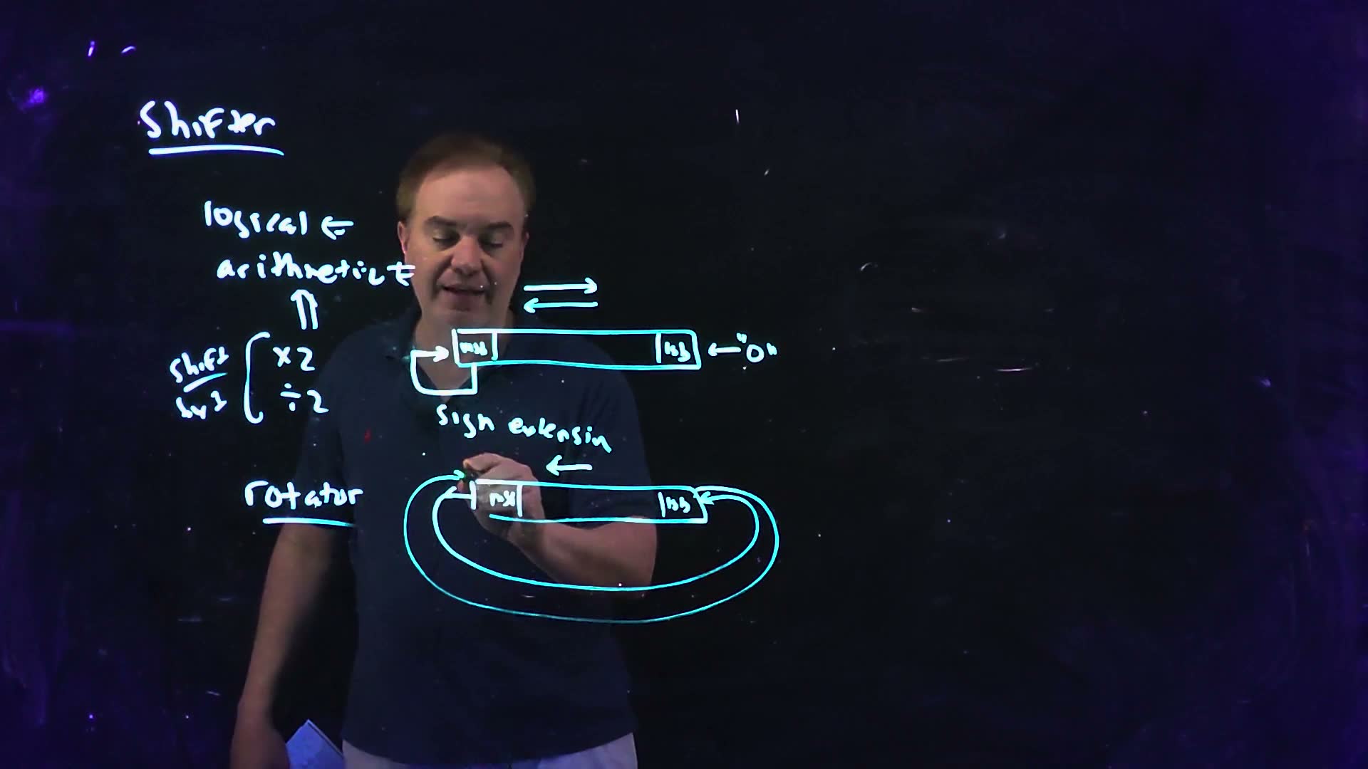
Fair copy of the board above (Lecture16 @ 22:11), mark for mark in its own layout. One pen (cyan) wrote the whole board, copied in black. The rotator box’s msb end and the outer loop’s arrowhead, under the lecturer’s hand here (he is finishing that arrowhead), are restored from the video at 22:14–22:40; the board is wiped by 23:16. The double arrow after “arithmetic” sits a little right of the board’s, because the typeset word runs wider.

One word shifted right by 2 three ways added. $A = 1011\,0110$ ($-74$−74 as a signed number), then, top to bottom: logically (two 0s enter at the MSB end: $0010\,1101 = 45$45, the sign is lost), arithmetically (two copies of the MSB enter: $1110\,1101 = -19$−19, the floor of $-74/4 = -18.5$−18.5), and rotated (the two bits that fall off the LSB end re-enter at the MSB end: $1010\,1101$10101101). The shaded cells are the bits each shift brings in.

An arithmetic right shiftadded

$$x \gg_{\text{arith}} n = \left\lfloor \frac{x}{2^n} \right\rfloor$$

Holds when: two's-complement words; a shift by n places, n smaller than the word length; it rounds toward −∞

Memorize or derive. Memorize the three fill rules: logical 0; arithmetic 0 on the left, a copy of the MSB on the right; rotate, the bit that fell off. Derive the rounding: each one-place shift halves the value and drops the LSB, which removes $\tfrac12$ when that bit was 1, so the result moves down, for a negative number away from zero.

A worked example (the board’s and an added one). Board: $-4 = 1111\,1100$ right by 1 with sign extension gives $1111\,1110 = -2$ (21:07). Added: the three shifts of $1011\,0110$ in step 4; check the arithmetic one by value, $\lfloor -74/4\rfloor = \lfloor -18.5\rfloor = -19$−19, and $1110\,1101 = -128 + 64 + 32 + 8 + 4 + 1 = -19$−19.

Traps.

• A logical right shift of a negative number. $1011\,0110$ ($-74$−74) becomes $0010\,1101 = 45$45: the sign is lost.
• Expecting $-3 \gg 1 = -1$−1. It is $-2$−2: $1111\,1101$ becomes $1111\,1110$11111110, and $\lfloor -1.5\rfloor = -2$−2. The shift rounds down, not toward zero.

Check yourself Rotate 1011 0110 right by 3.

$1101\,0110$11010110: the three bits that fall off the LSB end, 110, re-enter at the MSB end in the same order.

Check yourself What does an arithmetic right shift by 1 do to −1 = 1111 1111, and why is that the floor of −1/2?

Step 1: the bits move one place right and the MSB, 1, is copied in: $1111\,1111$ again, which is $-1$−1. Step 2: $-1/2 = -0.5$−0.5, and $\lfloor -0.5\rfloor = -1$−1: the shift rounds down, so $-1$ never shifts to 0.

8. The logarithmic shifter

You need

The 2:1 multiplexer (Chapter 10, §7). A select line picks one of two inputs and connects it to the output.

Pass transistors (Chapter 10, §4–§5). An NFET used as a switch passes a 0 fully but a 1 only up to $V_{DD} - V_T$VT​. An NFET and a PFET in parallel, gated by complementary signals (a transmission gate), pass both levels fully. A pass transistor has no supply of its own: its signal comes from the gate that drives it.

Stacks (Chapter 7, §5; Chapter 8, §10). Devices in series add their resistance, and the delay through a stack grows roughly as the square of its height; stacks taller than about three are avoided. Here the stack height of a path is the number of devices its charge passes in series: the driver’s device plus each pass transistor.

The kinds of shift (§7). A logical right shift fills the open MSB end with 0; an arithmetic one copies the MSB.

The kinds of shift (§7; Lecture16 @ 22:11, redrawn). Original figure ↑

The question. A shifter must move an 8-bit word right by any amount from 0 to 7. Building eight separate shifts and choosing one is wasteful. What is the cheapest structure that does every amount, and what does it cost in speed?

The building block (board, 22:55–26:31)

1. The specification (22:55–24:14) board. An “8-bit right shifter”, logical, whose shift amount is given fully encoded as a binary number $S_2S_1S_0$S2​S1​S0​: 111 shifts by 7, 010 by 2, 000 by 0, 110 by 6.
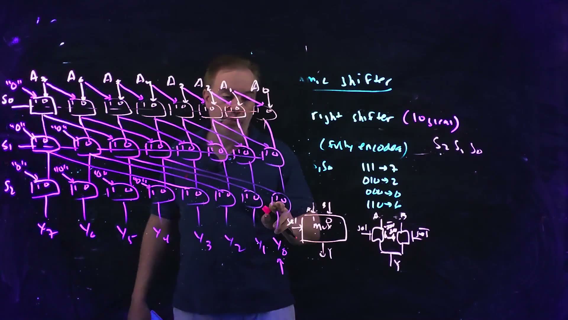
2. The 2:1 mux (25:15–26:31) board. A block with inputs “1” and “0”, a select sel and an output $Y$Y: “when select is a 1, it’s going to select this input”, the 1 input. As pass transistors it is two NFETs joined at $Y$Y, one gated by sel (passing input $A$A, the 1 input) and one by $\overline{\text{sel}}$ (passing $B$B). Each NFET passes a weak high, $V_{DD} - V_T$VT​; making each switch a transmission gate fixes that, “I don’t have to pay a VT drop”, at the cost of two more devices and the complement signals.

The 2:1 multiplexer the shifters are built from (Lecture16 @ 27:12). Left: the block: $Y$ is the “1” input when sel = 1 and the “0” input when sel = 0. Middle: the board’s pass-transistor form, two NFETs from $A$ (the 1 input) and $B$ (the 0 input) to $Y$Y, gated by sel and $\overline{\text{sel}}$sel; a high passes only to $V_{DD} - V_T$VT​. Right added (from the lecture’s spoken remark, 26:03–26:31): the complementary form, each NFET paired with a PFET on the complementary gate (a transmission gate), which passes a full $V_{DD}$ at the cost of two more devices.

The board (Lecture16 @ 27:12)

Lecture16 @ 27:12The first row of muxes, the encoded shift amount, the mux block and its pass-transistor form.

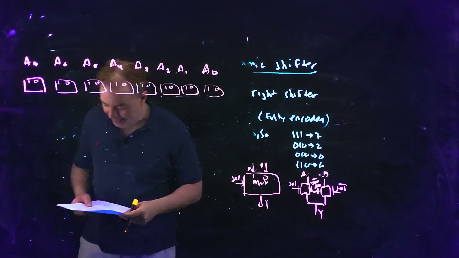
Fair copy of the board above (Lecture16 @ 27:12), mark for mark in its own layout. Magenta is the pink pen, which draws the shifter and the mux sketches; black is the cyan pen of the notes. The left of the board was wiped before 26:27, so the title “logarithmic shifter” and the line “S₂S₁S₀”, both whole at 24:09, are copied as they remain. The mux block’s top labels are A and B, written at 26:00 as the lecturer names the inputs; the 1 and 0 inside it mark which input each value of sel passes. At 26:15 each pass device was redrawn as a complementary pair, a loop of two channels, with small gate labels between the two (sel-bar and sel, set as read). The dash after “(fully encoded)” sits a little right of the board’s.

Three rows of muxes (board, 26:57–30:56)

1. Row $S_0$S0​: shift by 1 (26:57–28:31) board. Eight muxes, one per output bit, all selected by $S_0$S0​. Mux $i$ takes $A_i$ on its 0 input (straight down) and $A_{i+1}$ on its 1 input (diagonally from the left). Mux 7 has no $A_8$A8​, so its 1 input is a pad, 0, because the shift is logical.
2. Row $S_1$S1​: shift by 2 (28:58–29:41) board. The same, with the 1 input taken from two positions to the left of the row above; muxes 7 and 6 take 0 pads.
3. Row $S_2$S2​: shift by 4 (29:48–30:56) board. The 1 input comes from four positions to the left; muxes 7 to 4 take 0 pads. The outputs are $Y_7 \dots Y_0$Y7​…Y0​.
4. Why it covers every amount added. The rows shift by 1, 2 and 4 or not at all, so together they shift by $4S_2 + 2S_1 + S_0$S0​: the binary shift amount itself. Any amount from 0 to 7 is a sum of distinct powers of 2. That is why the select is encoded and why there are $\log_2 N$ rows: “logarithmic”.

The 8-bit logarithmic right shifter as the board builds it (Lecture16 @ 31:19, before the inverters), redrawn. Each box is a 2:1 multiplexer that passes its “1” input when its row’s select is 1 and its “0” input otherwise. Row $S_0$ shifts by 1, row $S_1$ by 2, row $S_2$ by 4: mux $i$ takes the bit straight above on its 0 input and the bit $2^k$ places to the left on its 1 input, and the inputs with no bit to the left take a 0 pad (a logical shift): one in row $S_0$S0​, two in row $S_1$S1​, four in row $S_2$S2​. The encoded amount $S_2S_1S_0$ is the shift: 101 shifts by 5.

The board (Lecture16 @ 32:54)

Lecture16 @ 32:54The logarithmic shifter complete, with inverters under the S₁ row and the outputs inverted.

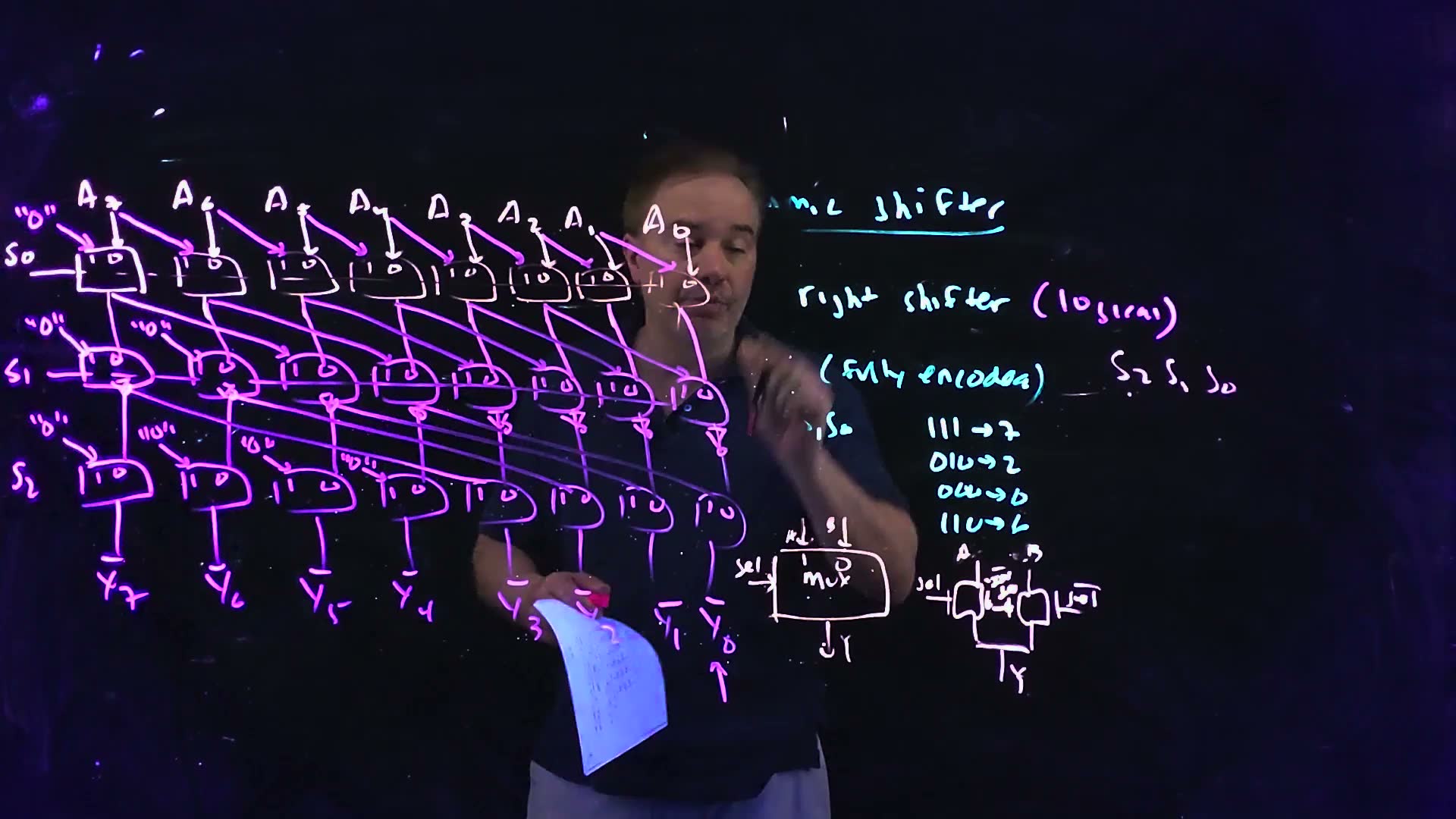
Fair copy of the board above (Lecture16 @ 32:54), mark for mark in its own layout, on the coordinates of the 27:12 copy. Magenta is the pink pen (the network, its pads and outputs, “(logical)”, “S₂ S₁ S₀” and the mux sketches); black is the cyan pen of the notes. $\overline{Y}_3$ to $\overline{Y}_1$Y1​, behind the lecturer’s hand and paper here, are restored from the video at 33:10, where the lower half is unchanged while he wipes the top. The bars over the outputs mark them inverted. Every pad is a quoted 0; the quote marks of the S₂ row’s second pad are written upright, so it reads like “10”. With the inverters, the S₂ row’s pads should become 1, as the lecturer says at 32:12, but the board keeps 0.

Stack height, and breaking it (board, 31:00–32:50)

1. Count the stack (31:00–31:30). A bit reaching $Y$ passes one pass transistor in each of the three rows, and before them the inverter that drives $A_i$Ai​: “My stack height here is at least four, which obviously isn’t very good” (31:30).
2. Break it with inverters (31:41–32:29) board. Put an inverter after each mux of the $S_1$ row. A path is then the driver and two pass devices (height 3), then the new inverter and one pass device (height 2). The outputs come out inverted, $\bar Y$Yˉ, as the board marks them.
3. The pads change (32:12). After the inverters, the $S_2$ row carries inverted data, so its pads must be inverted too: “I would need to also invert these zeros”. Its four pads become 1, though the board still shows them as 0.
4. The lesson. “You have to be very wary of the stack heights that you create when you use pass transistors” (32:45). Without buffers the height grows as $\log_2 N + 1$1; buffers every two or three rows keep it short, at the cost of an inverter delay each.

Stack height in the logarithmic shifter added (from the lecture’s spoken count, 31:00–32:42; the inverters’ place as on the board, Lecture16 @ 32:54). Top: the path from a driving inverter to an output passes one conducting pass NFET in each row ($S_0$S0​, $S_1$S1​, $S_2$S2​), so the driver’s pull-down sees four devices in series. Bottom: inverters after the $S_1$ row break the path into a stack of three (driver, $S_0$S0​, $S_1$S1​) and a stack of two (inverter, $S_2$S2​); the outputs come out inverted, $\overline{Y}$Y.

The arithmetic version (added)

1. What changes. An arithmetic right shift fills with copies of the MSB, so every pad must carry $A_{N-1}$ instead of 0.
2. Where the pad can come from. Straight from the input $A_{N-1}$AN−1​, in every row. An arithmetic right shift never changes the MSB (it copies it), so after any row the MSB is still $A_{N-1}$AN−1​.
3. At 4 bits. Two rows, $S_0$ (by 1) and $S_1$ (by 2); three pads, all wired to $A_3$A3​: mux 3’s 1 input in row $S_0$S0​, and muxes 3 and 2 in row $S_1$S1​. FN12-6 asks for the 8-bit version (seven pads); it is solved on the datapath practice page (FD1).

The logarithmic shifter made arithmetic, at 4 bits added: every input that the logical shifter ties to 0 is wired to $A_3$A3​, the sign bit, taken straight from the input (an arithmetic right shift never changes the MSB, so each row’s MSB is still $A_3$A3​). Row $S_0$ shifts by 1 and row $S_1$ by 2.

The logarithmic shifteradded

$$\begin{gathered} Y = A \gg (4S_2 + 2S_1 + S_0)\\ \log_2 N \text{ rows of } N \text{ muxes},\qquad \text{stack height} = \log_2 N + 1 \end{gathered}$$

Holds when: N a power of 2; row k shifts by 2^k when S_k = 1, its mux's 1 input taking the shifted bit; pads 0 (logical) or A_(N−1) (arithmetic); stack height without buffers, the driver included (the 8-bit count is spoken, 31:15)

Memorize or derive. Memorize the structure: row $k$ shifts by $2^k$ under $S_k$Sk​, the 1 input takes the shifted bit, and the pads are 0 or $A_{N-1}$AN−1​. Derive the counts and the stack height from it: one row per select bit, one mux per output bit, one pass device per row plus the driver.

A worked example added. $A = 1011\,0110$ (182 unsigned, $-74$ signed), $S = 101$ (shift by 5), row by row:

after row	shift	logical	arithmetic
input		1011 0110	1011 0110
$S_0 = 1$	1	0101 1011	1101 1011
$S_1 = 0$	0	0101 1011	1101 1011
$S_2 = 1$	4	0000 0101	1111 1101

Logical: $0000\,0101 = 5$5, and $\lfloor 182/32\rfloor = 5$5. Arithmetic: $1111\,1101 = -3$−3, and $\lfloor -74/32\rfloor = \lfloor -2.3125\rfloor = -3$−3.

Traps.

• Inverting the row outputs but leaving the next row’s pads at 0. After the inversion a 0 pad stands for a true 1: a shift by 4 would fill the top four bits with 1s.
• Swapping the mux inputs. With the board’s convention the 1 input takes the shifted bit (FN12-6’s $y = ac + b\bar c$ has $a$ as that input). Wired the other way, $S = 000$ shifts by 7.

Check yourself With S = 011, which input bit reaches Y₂?

$A_5$A5​: the amount is $2 + 1 = 3$3, so $Y_2 = A_{2+3}$A2+3​. The $S_0$ row moves $A_5$ to position 4, the $S_1$ row moves it on to position 2, and the $S_2$ row passes it straight down.

Check yourself A 16-bit logarithmic shifter: how many rows and muxes, and what is its stack height without buffers?

Step 1: $\log_2 16 = 4$ rows ($S_3S_2S_1S_0$S3​S2​S1​S0​, shifts 1, 2, 4, 8) of 16 muxes: 64 muxes. Step 2: the driver plus one pass device per row: $4 + 1 = 5$5, too tall; an inverter after the second row gives 3 and 3.

9. The barrel shifter and one-hot selects

You need

Static, ratioed, floating (Chapter 10, §7). A pass-transistor multiplexer is static only when exactly one select is on: its output is then connected to exactly one driven input. Two selects on with different data make a fight, whose result depends on the ratio of the drivers’ strengths (ratioed logic). No select on leaves the output floating, held only by its own capacitance. Selects with exactly one 1 are called one-hot or orthogonal; a decoder makes them from a binary number (Chapter 19 builds decoders).

Sign extension (§7). An arithmetic right shift fills the open MSB end with copies of the MSB.

The kinds of shift (§7). Original figure ↑

The logarithmic shifter (§8): $\log_2 N$ rows of 2:1 muxes, a stack height of $\log_2 N + 1$1.

The 2:1 pass-transistor multiplexer (§8). Original figure ↑

The question. The logarithmic shifter puts a pass device per row on every path. Can each output be connected to the input it needs through one pass transistor, and what does that demand of the select lines?

A 4-bit arithmetic right barrel shifter (board, 33:10–41:38)

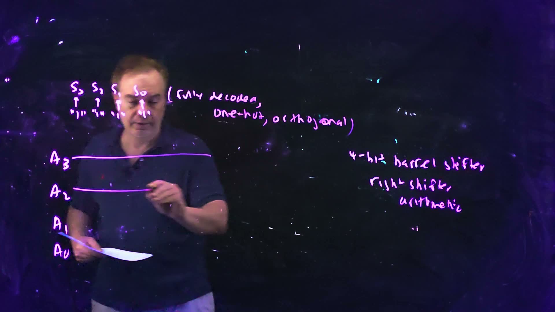
1. The select (33:10–35:19) board. Four lines $S_3S_2S_1S_0$S3​S2​S1​S0​, “fully decoded, one-hot, orthogonal”: exactly one is 1, and $S_k = 1$ means shift by $k$k. “If that’s not true, then the circuit will not be static. It’ll be ratioed” (35:19).
2. The lines (35:19–36:33) board. Inputs $A_3 \dots A_0$ run across from the left, outputs $B_3 \dots B_0$ leave to the right; a right shift, arithmetic, by 0 to 3.
3. The shift devices (37:04–39:07) board. One NFET per output and select. Under $S_0$S0​, each $B_j$ connects to $A_j$Aj​; under $S_1$S1​, $B_0$ to $A_1$A1​, $B_1$ to $A_2$A2​, $B_2$ to $A_3$A3​; under $S_2$S2​, $B_0$ to $A_2$ and $B_1$ to $A_3$A3​; under $S_3$S3​, $B_0$ to $A_3$A3​.
4. The sign-extension devices (39:18–41:13) board. The outputs left without a source get the MSB: under $S_1$S1​, $B_3$ to $A_3$A3​; under $S_2$S2​, $B_3$ and $B_2$ to $A_3$A3​; under $S_3$S3​, $B_3$B3​, $B_2$ and $B_1$ to $A_3$A3​. The rule in one line added: under $S_k$Sk​, $B_j$ connects to $A_{\min(j+k,\,3)}$Amin(j+k,3)​. Sixteen devices, six of them sign extension (those with $j + k > 3$3; the board rings them with a cyan arc).
5. Stack height (41:38). The driver and one pass transistor: 2, for any shift.

The 4-bit arithmetic right barrel shifter (Lecture16 @ 42:04), redrawn as a clean crossbar; the board’s own routing is kept in its fair copy. The columns run $S_3$ to $S_0$S0​, as the board’s header. Each output $B_j$ connects through one NFET per select line $S_k$ to the input $A_{\min(j+k,\,3)}$Amin(j+k,3)​: exactly one select is on (one-hot), so each output passes the input $k$ places to its left through a single device. The six devices in the dashed outline connect outputs to $A_3$ beyond the word’s end: they copy the sign bit (sign extension). For example, $A = 1010$ with $S_1$ on gives $B = 1101$1101: $-6 \div 2 = -3$−3.

The board (Lecture16 @ 42:04)

Lecture16 @ 42:04The 4-bit arithmetic barrel shifter: one-hot selects, sixteen pass transistors, the sign-extension devices ringed.

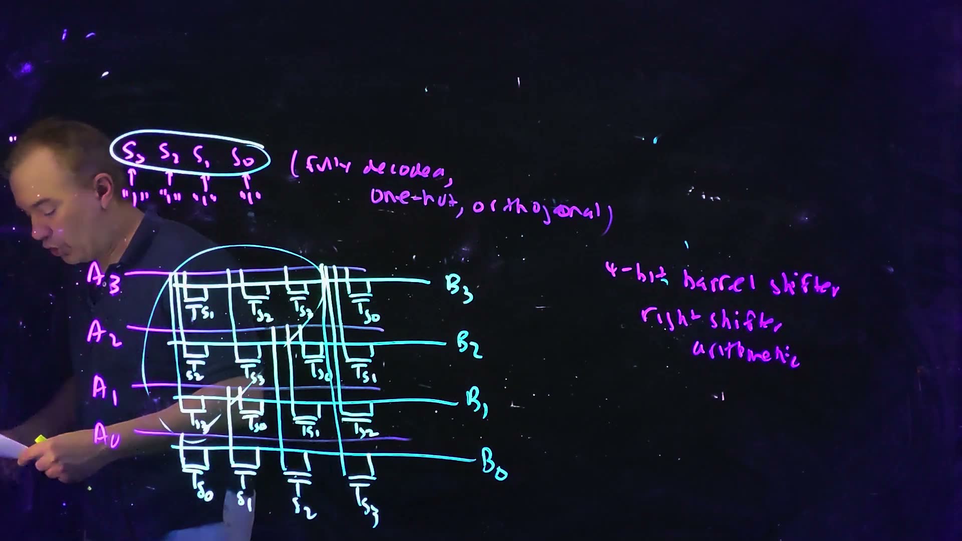
Fair copy of the board above (Lecture16 @ 42:04), mark for mark in its own layout, with the board’s own routing of the vertical wires. Magenta is the violet pen: the input lines $A_3 \dots A_0$ with their labels, and both notes. Teal is the cyan pen: the output lines $B_3 \dots B_0$ with their labels, and the large arc. Black is the white pen: the select ring with its arrows and “1”s, the sixteen pass transistors with their gate labels, and the vertical wires, each running from its input line to one device. The diagonal below the arc’s right end (cyan at the top, two white dashes lower down) cuts down between the devices to the arc’s lower end: with the arc it encloses the six sign-extension devices. In the ring the lecturer’s $S_3$ looks like “S>”; the routing checks out device by device against $B_j = A_{\min(j+k,\,3)}$Amin(j+k,3)​. The input labels are read on 41:42, where the sheet in his hand is clear of $A_0$A0​. The white pen retraces the output lines inside the array; the copy draws them in teal throughout.

Why the select must be one-hot (spoken 35:19, 41:13; floating case added)

1. One select on. Each output has exactly one conducting device, to one driven input: a static circuit. With $S_1$ on and $A = 1010$1010, $B_1$ connects to $A_2 = 0$0.
2. Two selects on. $S_0$ and $S_1$ together join $B_1$ to both $A_1$ and $A_2$A2​. If they differ, one driver pulls up and the other down: a fight, settled by the ratio of their strengths. With $S_0$ and $S_1$ both on, 14 of the 16 possible input words make at least one output fight (only 0000 and 1111 do not).
3. No select on added. Every device is off, so each output floats: it keeps whatever charge it had, a dynamic node.
4. So the select lines come from a decoder, which guarantees exactly one 1.

One output of the barrel shifter, $B_1$B1​, with its four devices added. (a) Exactly one select on ($S_1$S1​): one device conducts and $B_1 = A_2$A2​. (b) Two selects on ($S_0$S0​ and $S_1$S1​) with $A_1 = 0$ and $A_2 = 1$1: two inputs drive $B_1$ against each other, so its level depends on the devices’ strengths (ratioed). (c) No select on: nothing drives $B_1$B1​, which floats and holds whatever charge it had (dynamic). Only the one-hot case is static.

Against the logarithmic shifter added. The barrel shifter has one pass device per path but $N^2$ devices and $N$ one-hot select lines, plus the decoder that makes them. The logarithmic shifter has $\log_2 N$ pass devices per path, $N\log_2 N$ muxes (two NFETs each) and only $\log_2 N$ encoded select lines.

$N$ bits	4	8	16	32
barrel: NFETs	16	64	256	1024
barrel: select lines	4	8	16	32
logarithmic: muxes (NFETs)	8 (16)	24 (48)	64 (128)	160 (320)
logarithmic: select lines	2	3	4	5

The barrel shifter (arithmetic right)added

$$\begin{gathered} \text{under } S_k:\quad B_j = A_{\min(j+k,\ N-1)}\\ N^2 \text{ devices, of which } \tfrac{N(N-1)}{2} \text{ sign extension} \end{gathered}$$

Holds when: one-hot selects S₀ … S_(N−1), S_k = shift by k; one NFET per (j, k); the 4-bit device list is the board's, the general rule added

Memorize or derive. Memorize the one-hot rule and its reason (two on fight, none on float). Derive any output’s device list from $A_{\min(j+k,N-1)}$Amin(j+k,N−1)​, and the counts from the grid.

A worked example added. $A = 1010$ ($-6$−6), $S_1$ on: $B_3 = A_3 = 1$ (sign extension), $B_2 = A_3 = 1$1, $B_1 = A_2 = 0$0, $B_0 = A_1 = 1$1. So $B = 1101 = -3$−3, and $\lfloor -6/2\rfloor = -3$−3.

Traps.

• Driving the select lines from a binary amount. Wired to $S_0$ and $S_1$S1​, the 2-bit amount 3 (binary 11) turns both on at once: a fight. A 2-to-4 decoder must come first.
• Leaving out the sign-extension devices. Then on a shift by $k$ the top $k$ outputs have no path at all: they float, which is not even a logical shift.

Check yourself Which input reaches B₁ when S₂ is on?

$A_3$A3​: $\min(1 + 2, 3) = 3$3. A right shift by 2 puts bit 3 at position 1.

Check yourself An 8-bit arithmetic right barrel shifter: how many devices and select lines does it need, and how many of the devices are sign extension?

Step 1: one NFET per output and select: $8 \times 8 = 64$ devices, with 8 one-hot select lines. Step 2: sign extension where $j + k > 7$7: output $B_7$ has 7 such devices ($k = 1 \dots 7$k=1…7), $B_6$ has 6, down to $B_1$ with 1, so $1 + 2 + \dots + 7 = 28$28.

10. Other datapath blocks, control logic and the synthesis flow (background for the final)

You need

The three kinds of circuit (Chapter 15, §11). A processor is datapath (structured, often custom), control logic (“random”, unstructured) and arrays (memory, structured).

Static timing analysis (Chapter 14, §8). A tool checks every path between storage elements against the clock period, without simulating patterns.

The question. The adders and shifters are hand-built, bit by bit. The control logic that steers them cannot be: what is it, and how is it built instead?

From the datapath to control logic (board, 42:02–54:46)

1. Other datapath blocks (42:02–42:32). Fixed-point multipliers, “even dividers”, and logic units are datapath blocks too; the course names them only. The adder and the shifter are the two most critical.
2. Control logic (42:53–44:20) board. Back to the taxonomy: datapath, control, memory and arrays. Control logic is “random” logic: “All the term random means is that it’s not structured” (43:38). It also changes up to the last minute, since most of a processor’s bug fixes land in it before tape-out (“rapid changes”). So it is built with CAD automation, a semi-custom flow.
3. Two strategies (44:20–47:05) board. Unstructured: multi-level logic, made by a synthesis and place-and-route (P&R) flow. Structured: two-level sum-of-products (SOP) logic in a programmable logic array (PLA). A PLA is regular and has good heuristic optimization tools; its disadvantage is area. It “comes and goes in vogue”.
4. The synthesis flow (47:34–52:11) board. An RTL description (Verilog or VHDL) goes into logic synthesis (for example Synopsys Design Compiler), which maps it onto a standard-cell library of gates (NANDs, NORs, AOIs: channel-connected components) and writes a netlist. Place-and-route puts the cells’ layouts in rows and wires them up (“a rat’s nest”) and writes the GDS file for the foundry. Every cell has the same height, between M1 supply rails (vdd! and gnd!) that join up along a row; widths vary, each gate comes in several drive strengths (“power levels”), and gaps are filled with filler cells. Static timing analysis with the real wire loads then sends the design back to synthesis until it meets timing. “We’re not going to be using these in this class” (52:11).
5. What the course uses: PLAs (52:11–54:46). The design project builds its processor’s control logic as a PLA. The logic is written as a sum of products: each product term is an AND of input literals (a variable or its complement), and each output is an OR of product terms. An RTL description converts easily into such a sum-of-products table and back. When the lecturer was at IBM, some argued that all logic should be captured in these tables instead of in VHDL or Verilog, an idea that “never caught on” (53:58–54:32). Chapter 18 §1 takes up the lecture’s example and turns its AND–OR form into the NOR–NOR form a PLA is built from.

The two ways to build control logic, redrawn from the board (Lecture16 @ 46:44). Control (“random”, unstructured logic) changes quickly during a design, so it is built semi-custom, with CAD automation. Two routes: unstructured, as multi-level logic through logic synthesis and place-and-route (P&R); or structured, as a programmable logic array (PLA), a two-level sum-of-products (SOP) form.

The board (Lecture16 @ 46:44)

Lecture16 @ 46:44Control logic: random logic, rapid changes, semi-custom; multi-level synthesis or a two-level PLA.

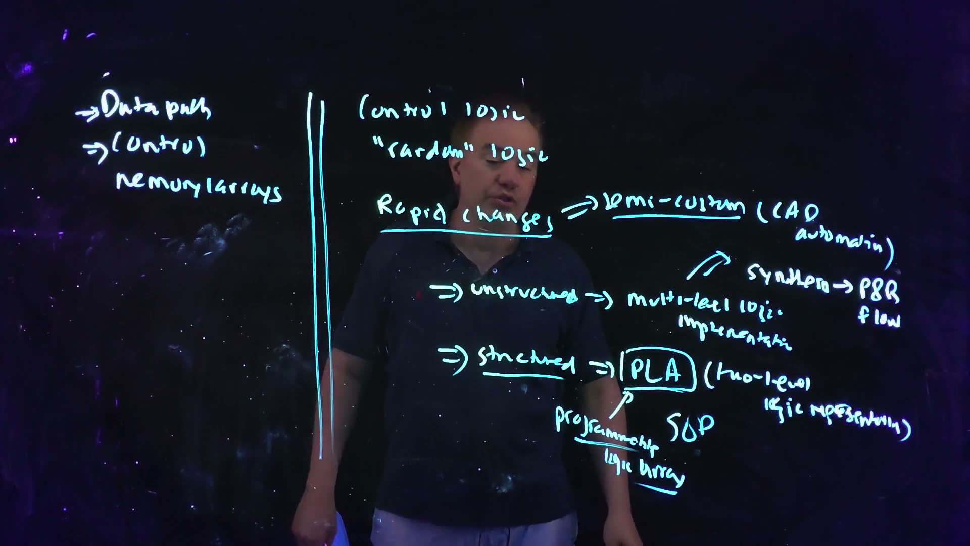
Fair copy of the board above (Lecture16 @ 46:44), mark for mark in its own layout. All black: a white pen wrote the words, and a cyan pen drew the right-hand rule, the underlines, the up arrow, the box round PLA and “SOP”. The two pens alternate through the topic without marking a separate layer, and by this frame the camera’s colour has tinted the whole board cyan. The hand writes some words small (“unstructured”, “implementation”, “programmable logic array”), and they are set smaller here; the bracket after “automation” moves right to clear the typeset word.

The semi-custom flow, redrawn from the board (Lecture16 @ 52:19). RTL, written in Verilog or VHDL, goes to logic synthesis (the lecture names Synopsys Design Compiler), which maps it onto the gates of a standard-cell library and writes a netlist; place-and-route (P&R) places the cells’ layouts and wires them, and writes the GDS file for the mask shop; static timing analysis (STA) with the wires’ parasitics loops back to synthesis until timing closes. Below: standard cells all have one height $h$h, so they sit in rows between shared metal-1 rails (vdd! above, gnd! below); a filler cell (hatched) fills a gap in a row.

The board (Lecture16 @ 52:19)

Lecture16 @ 52:19The synthesis and place-and-route flow, standard-cell rows and the cell's supply rails.

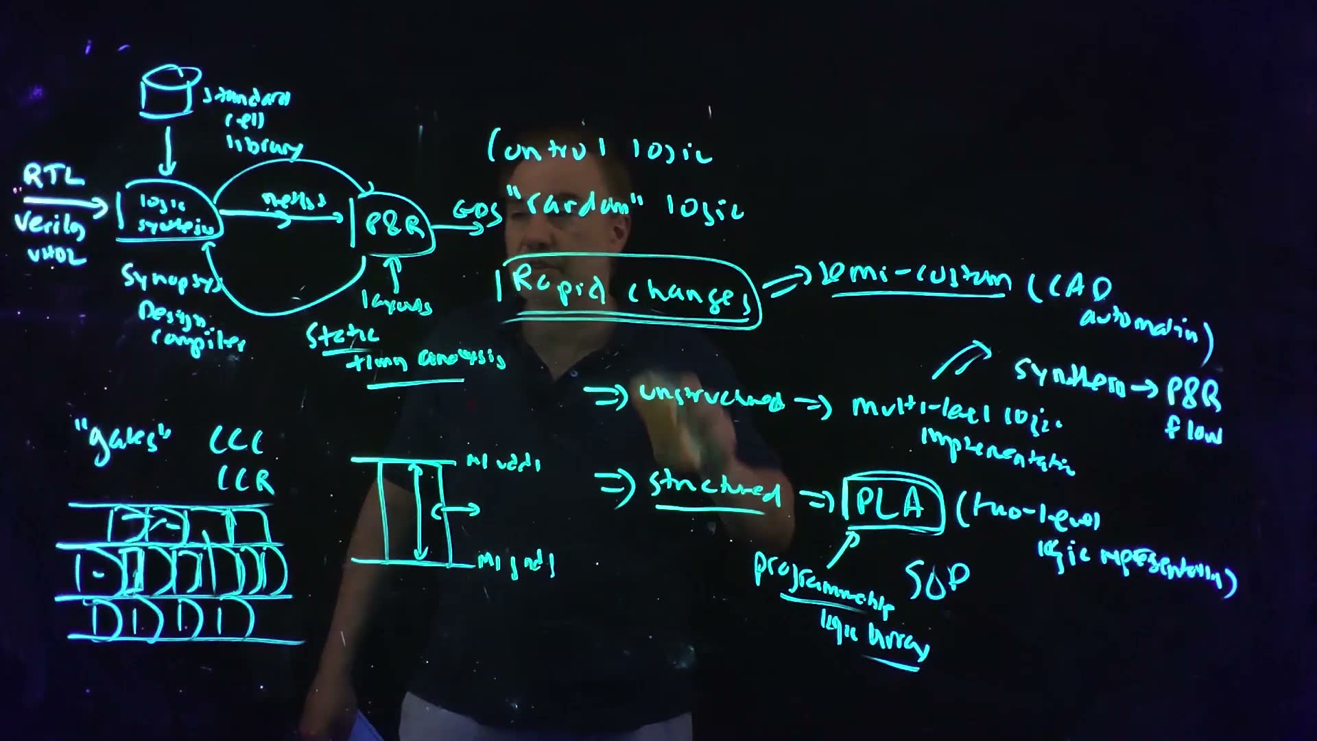
Fair copy of the board above (Lecture16 @ 52:19), mark for mark in its own layout. All black: by now the camera shows a single colour, and the white and cyan pens of 46:44 cannot be told apart. The right half is the 46:44 board with “Rapid changes” now boxed; the taxonomy and the double rule at the left are erased, and the design flow, the standard-cell rows and a cell’s outline take their place. The lecturer’s hand, holding the eraser over “unstructured”, hides nothing new: every stroke matches 51:57, where it is clear. The loop under the flow, labelled “static timing analysis”, carries the results of P&R back into logic synthesis. The cell rows are copied cell by cell, each a bar and a D-shaped outline as the hand drew them; the right half’s words are set a size smaller than at 46:44, since this copy is drawn at a smaller scale.

Check yourself Why does control logic suit an automated flow better than a hand layout, and what does a PLA give up for its regularity?

Step 1: control logic is unstructured and changes late and often, since most bug fixes land in it before tape-out; an automated flow can redo it overnight, while a hand layout would have to be redrawn. Step 2: a PLA’s regular two-level array is easy to generate and optimize, but it can waste area compared with multi-level logic.

Check yourself An RTL statement sets y = (a and b) or (not c). Write y as a sum of products, and on how many of the eight input combinations is y = 1?

Step 1: $y = ab + \bar c$cˉ: two product terms, $ab$ (an AND of two literals) and $\bar c$ (one complemented literal), ORed. Step 2: $\bar c = 1$ on the 4 combinations with $c = 0$0, and $ab$ adds the one with $a = b = 1$1, $c = 1$1: 5 of 8. Check: $y = 0$ needs $c = 1$ and $ab = 0$0, which is 3 combinations, and $8 - 3 = 5$5.

On the exam

Two past-final parts rest directly on this chapter, both 15-point block drawings, and both with a twist the lecture does not draw. A third, FN12-10a, uses the sum-of-products form that §10 introduces; it is Chapter 18’s.

Part	Points	What it asks	Sections
FN17-8	15	the block diagram of an 8-bit parallel adder from PG generators, radix-two lookahead elements and sum generators, and its critical path	§1, §2, §3, §6 (§5 for the levels); with Chapter 16 §9, §12, §13
FN12-6	15	the block-level schematic of an 8-bit arithmetic right shifter from 2:1 muxes ($y = ac + b\bar c$y=bcˉ), with a 3-bit shift amount	§7, §8 (the arithmetic pads); §9 for contrast
FN12-10a	9	the functions of a NOR–NOR PLA	Chapter 18 §1 onward; §10 here names the sum-of-products form only

All three are solved, with their own figures and keys, on the datapath practice page (FD1). What this chapter prepares:

• FN17-8. The three blocks are Chapter 16’s PG cell, the radix-2 element (§1) and the sum XOR. The network is any radix-2 network over positions 0 to 8, the carry-in entering as $(c_{in}, 0)$(cin​,0): Kogge–Stone (§3) or Brent–Kung (§4). Each sum takes the carry of the bit below it, $s_k = p_k\oplus G_{k-1:0}$Gk−1:0​, and $s_1 = p_1\oplus c_{in}$cin​: wiring $s_k$ to its own column’s $G_{k:0}$ is the trap of §6. The critical path runs PG, up the network to the carry the top sum needs, and through that sum, or up to $c_{out}$ (§6). At the finals’ pace of 0.7–0.9 minutes a point, it is a 10–14 minute part.
• FN12-6. The lecture’s logarithmic shifter (§8) is logical; the arithmetic version fills every pad with $A_7$ (§8, the arithmetic steps), and the mux’s $a$ input takes the shifted bit. Also a 10–14 minute part.

Memorize.

• The element $(G_{hi} + P_{hi}G_{lo},\ P_{hi}P_{lo})$Phi​Glo​, Phi​Plo​), higher span first: bracket freely, never swap.
• $C_k = G_{k:0}$ with $c_{in}$ entered as $(c_{in}, 0)$(cin​,0); $s_k = p_k\oplus C_{k-1}$Ck−1​; $c_{out} = C_N$CN​.
• Kogge–Stone’s rule (column $m$ reaches $2^{m-1}$ rows down) and Brent–Kung’s shape (pairs, then 2:0, 4:0, 8:0 from position 0, then fill in).
• Kogge–Stone is the faster, Brent–Kung the smaller; Brent–Kung’s cost is levels and irregular fan-out.
• The three kinds of shift and their fill bits; an arithmetic right shift rounds down.
• The logarithmic shifter: row $k$ shifts by $2^k$ under $S_k$Sk​; stack height $\log_2 N + 1$ unless buffered.
• The barrel shifter’s one-hot select and why (two on fight, none on float).
• The two ways to build control logic: synthesis and P&R, or a PLA.

Derive (with the path).

• Associativity. Expand $(x\circ y)\circ z$ and $x\circ(y\circ z)$z): both are $(g_x + p_xg_y + p_xp_yg_z,\ p_xp_yp_z)$px​py​gz​, px​py​pz​).
• The lower bound. Each element at most doubles the positions a signal depends on: $\lceil\log_2(k + 1)\rceil$ levels for $C_k$Ck​.
• Counts at a given width. Kogge–Stone: $N + 1 - 2^{m-1}$ elements in column $m$ for $N$ bits. Brent–Kung: draw it.
• A critical path. $t_{PG}$tPG​, plus the depth of $C_{N-1}$ times $t_e$te​, plus $t_{sum}$tsum​; and $t_{PG}$ plus the depth of $C_N$ times $t_e$ for $c_{out}$cout​.
• The arithmetic pads. $A_{N-1}$AN−1​, straight from the input, because an arithmetic right shift never changes the MSB.
• A barrel output’s devices. Under $S_k$Sk​, $B_j = A_{\min(j+k,N-1)}$Amin(j+k,N−1)​.

Method cards. The playbook’s cards: “prefix adder” (recognize PG, lookahead-element and sum blocks, or “draw the critical path”; moves: PG, a network over positions 0 to $N$N, sums from the carry below, mark the deepest path; traps: the sum index and $p = a\oplus b$b) and “shifter from muxes” (recognize a mux block and an encoded shift amount; moves: one row per select bit shifting by $2^k$2k, the shifted bit on the select-1 input, the pads; traps: logical against arithmetic pads, and the stack height). FN12-10a’s card belongs to Chapter 18.

The lecture’s boards

The boards of Lecture 16 used in this chapter (23 frames)

Lecture16 @ 00:18 the recap column being written

Lecture16 @ 02:43 the radix-2 element being written

Lecture16 @ 03:32 Radix-2 tree adders: Brent-Kung, Kogge-Stone, the element

Lecture16 @ 05:24 Kogge-Stone: the inputs and the first element

Lecture16 @ 08:24 Kogge-Stone through column 2

Lecture16 @ 09:39 Kogge-Stone through column 3

Lecture16 @ 10:41 Kogge-Stone complete

Lecture16 @ 13:44 Brent-Kung: the inputs and 0–1

Lecture16 @ 15:26 Brent-Kung through 0–3

Lecture16 @ 17:26 Brent-Kung complete, C₁ uncovered

Lecture16 @ 17:54 Brent-Kung, titled

Lecture16 @ 20:31 the logical and arithmetic word box

Lecture16 @ 22:11 shifters: logical, arithmetic, rotator

Lecture16 @ 24:09 logarithmic shifter: the encoded shift amount

Lecture16 @ 27:12 the first mux row; the mux and its pass-transistor form

Lecture16 @ 31:19 the logarithmic shifter, before the inverters

Lecture16 @ 32:54 the logarithmic shifter with inverters

Lecture16 @ 36:33 the barrel shifter lines before the devices

Lecture16 @ 39:42 the barrel shift devices, before sign extension

Lecture16 @ 42:04 the barrel shifter complete

Lecture16 @ 43:29 datapath, control, memory

Lecture16 @ 46:44 control logic: synthesis or PLA

Lecture16 @ 52:19 the synthesis and place-and-route flow