5. Body effect, capacitance and delay

Lecture 4 gave the transistor’s current. Lecture 5 finishes the device picture with three more things a circuit designer needs. First, the body effect: what happens to the threshold when the source is not at the body’s potential. Second, the transistor’s capacitances: digital circuits work by charging and discharging capacitors, so the capacitance matters as much as the current. Third, speed: the lecture defines the transistor’s unity-gain frequency $f_T$fT​, shows that it comes down to the time carriers take to cross the channel, and then uses that same transit time to estimate how fast an inverter switches (the fan-out-of-one and fan-out-of-four delays).

After this chapter you can:

1. explain the body effect, and calculate the threshold with a source-to-body bias;
2. split a transistor’s capacitance into intrinsic parts (by region of operation) and extrinsic parts (overlap and junction), and estimate wire capacitance;
3. choose a layout that shares diffusions so less junction capacitance sits on a switching node, and explain how wells are tied to the supplies;
4. derive $f_T = g_m/(2\pi C_{gs})$ from the small-signal model and show that $f_T = 1/(2\pi\tau_{tr})$1/(2πτtr​), with $\tau_{tr} = L/v_{sat}$L/vsat​;
5. estimate the delay of one NFET discharging another, and the FO1 and FO4 inverter delays, from the transit time.

Boxes and equations marked board were written in the lecture. Parts marked added are explanations or examples this guide adds.

Before you start

You need these ideas from earlier chapters. Each is restated here.

• Threshold (Chapter 3). $V_T = V_{FB} + 2\phi_F + Q_{bulk}/C_{ox}$Qbulk​/Cox​, with $\phi_F = \frac{kT}{q}\ln\frac{N_A}{n_i}$ and the depletion charge $Q_{bulk} = \sqrt{2qN_A\kappa_s\varepsilon_0\,(2\phi_F)}$ per area.
• Junction capacitance (Chapter 3). A reverse-biased junction is a capacitor, $C_j = \kappa_s\varepsilon_0/W$ per area. Its depletion width $W$ grows as $\sqrt{V_{bi} + V_R}$Vbi​+VR​​, so $C_j$ falls as the reverse bias $V_R$ rises.
• Oxide capacitance (Chapter 3). $C_{ox} = \kappa_{ox}\varepsilon_0/t_{ox}$ per area, $\kappa_{ox} = 3.9$3.9.
• Velocity-saturated current (Chapter 4). For short channels, $I_{DSAT} = C_{ox}Wv_{sat}(V_{GS} - V_T)$VT​): charge per area $C_{ox}(V_{GS} - V_T)$VT​), moving at $v_{sat}$vsat​, across a width $W$W.
• Holes are slower (Chapter 4). $v_{sat} \approx 10^7\,\mathrm{cm/s}$ for electrons and about half that for holes.
• Delay is $CV/I$ (Chapter 4, Dennard scaling). The time to charge a capacitance $C$ through a voltage $V$ with a current $I$I.
• Constants: $\varepsilon_0 = 8.85\times10^{-14}\,\mathrm{F/cm}$10−14F/cm, $\kappa_s = 11.7$11.7, $q = 1.6\times10^{-19}\,\mathrm{C}$10−19C, $kT/q = 26\,\mathrm{mV}$26mV. And $1\,\mathrm{fF} = 10^{-15}\,\mathrm{F}$10−15F.

Notation. The board writes the bulk potential as $|\phi_P|$ or $|\phi_F|$∣ϕF​∣; this guide keeps Chapter 3’s $\phi_F$ϕF​. $C_{gs}$Cgs​, $C_{gd}$ and $C_{gb}$ are gate-to-source, gate-to-drain and gate-to-body capacitances; $C_g$ and $C_d$ are a transistor’s total gate and drain capacitance; $\eta = C_g/C_d$Cg​/Cd​. $\tau_{tr}$ is the transit time.

One device for the examples. added Chapter 4’s NMOS again, not a fit to a real process: $W = 1\,\mu\mathrm{m}$1μm, $L = 0.25\,\mu\mathrm{m}$0.25μm, $t_{ox} = 5.4\,\mathrm{nm}$5.4nm, $v_{sat} = 10^7\,\mathrm{cm/s}$107cm/s, $V_T = 0.5\,\mathrm{V}$0.5V, $V_{DD} = 2.5\,\mathrm{V}$2.5V. For the body effect it has Chapter 3’s body doping, $N_A = 10^{17}\,\mathrm{cm^{-3}}$1017cm−3, and a flat-band voltage that makes $V_T = 0.5\,\mathrm{V}$ when source and body are at the same potential. Its drain is an $n^+$ region with $N_D = 10^{20}\,\mathrm{cm^{-3}}$1020cm−3.

1. The body effect

The idea. If the source sits above the body, the depletion region under the gate has to be deeper before the channel forms. More depletion charge means a higher threshold, and so less overdrive and less current.

Lecture05 @ 08:09The body effect: the device with V_SB (top left), the stack where it happens (centre), the threshold with V_SB, and the bigger Q_bulk (right).

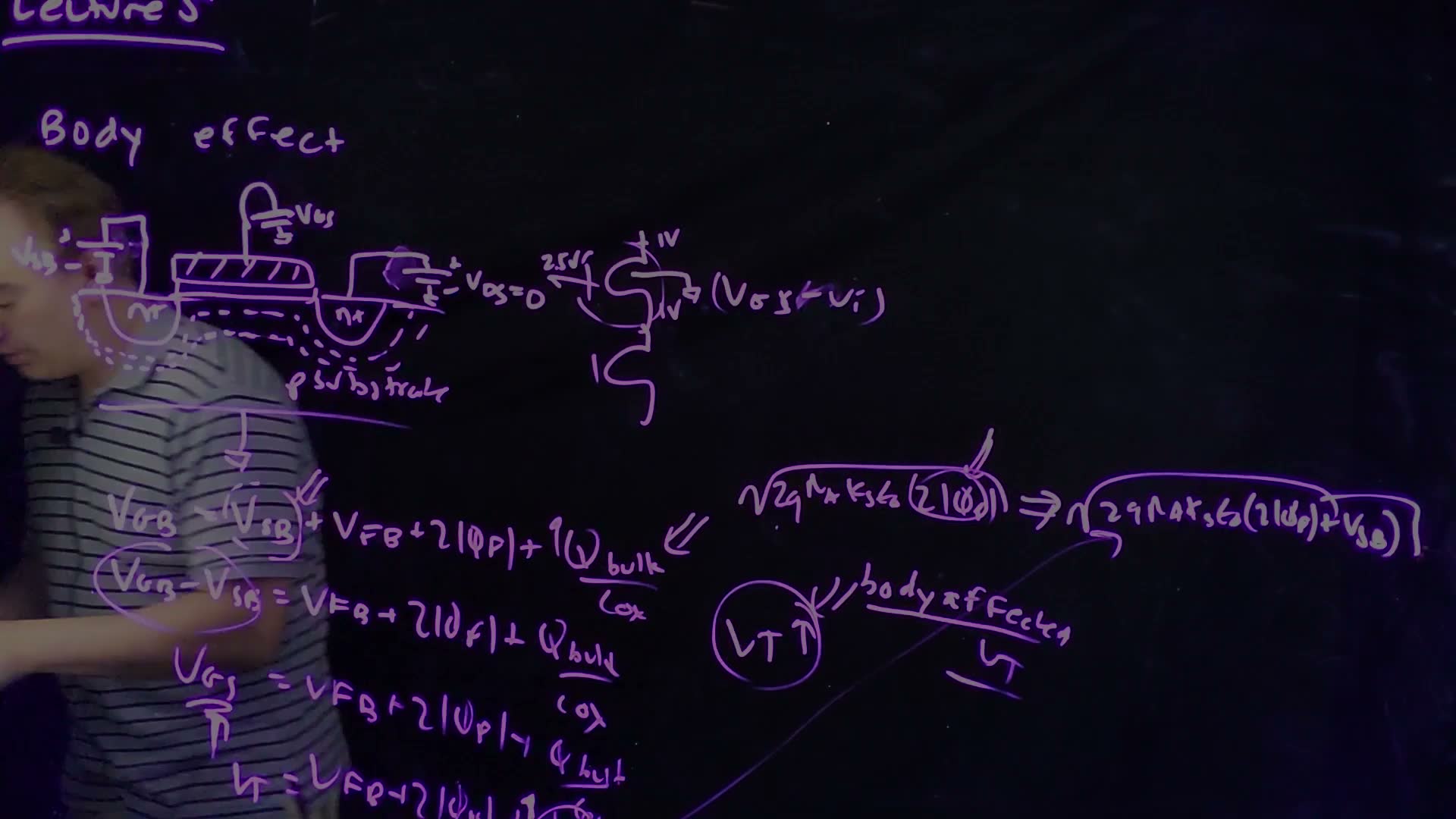
When the source is not at the body

Until now the source and the body were both grounded (00:40). In general they need not be: the lecture allows a source-to-body bias $V_{SB}$ (01:09). It must be applied as a reverse bias, positive on the $n^+$ source with respect to the p body, so the source junction never conducts (01:37).

This is not an exotic case. Picture two NMOS transistors in a stack, one above the other, with the body of both grounded (02:03–02:56). When the circuit runs, the node between them can sit at, say, 1 V. Then the upper transistor’s source is at 1 V while its body is at 0 V: $V_{SB} = 1\,\mathrm{V}$1V. “This scenario happens in circuits all the time.”

The threshold with a body bias

Set $V_{DS} = 0$ and look only at the threshold (02:56). The MOS structure is really controlled by the gate-to-body voltage (03:22). The derivation:

Threshold with a source-to-body bias (board, 03:22–05:56)

1. Write the threshold condition from the gate to the body board: $V_{GB} = V_{SB} + V_{FB} + 2\phi_F + \dfrac{Q_{bulk}}{C_{ox}}$Cox​Qbulk​​. The first term is new: the channel connects to the source, which sits $V_{SB}$ above the body.
2. Move $V_{SB}$ to the left board: $V_{GB} - V_{SB} = V_{FB} + 2\phi_F + \dfrac{Q_{bulk}}{C_{ox}}$Cox​Qbulk​​.
3. The left side is the gate-to-source voltage added: $V_{GB} - V_{SB} = (V_G - V_B) - (V_S - V_B) = V_{GS}$VGS​. So the threshold, as always measured gate to source, is $V_T = V_{FB} + 2\phi_F + Q_{bulk}/C_{ox}$ board: the same formula as before.
4. The difference is inside $Q_{bulk}$ (04:16). The reverse bias makes every depletion region wider: under the source, under the drain and under the gate. The depletion region under the gate now holds $2\phi_F + V_{SB}$ instead of $2\phi_F$ board: $Q_{bulk} = \sqrt{2qN_A\kappa_s\varepsilon_0\,(2\phi_F + V_{SB})}$2qNA​κs​ε0​(2ϕF​+VSB​)​.
5. A bigger $Q_{bulk}$ gives a bigger $V_T$ (05:56). This is the body-affected $V_T$VT​.

At 04:45 the speech says the old $Q_{bulk}$ was “twice $qN_A\kappa_s\varepsilon_0$ over twice $\phi_F$ϕF​”. The board multiplies, as Chapter 3 does: $\sqrt{2qN_A\kappa_s\varepsilon_0\,(2\phi_F)}$2qNA​κs​ε0​(2ϕF​)​.

Body effectboard

$$V_T = V_{FB} + 2\phi_F + \frac{Q_{bulk}}{C_{ox}}$$$$Q_{bulk} = \sqrt{2qN_A\kappa_s\varepsilon_0\,(2\phi_F + V_{SB})}$$

At $V_{SB} = 0$ this is Chapter 3’s threshold, $V_{T0}$VT0​.

Holds when: V_SB ≥ 0 (source–body junction reverse-biased); uniform body doping; V_T measured gate to source

A shortcut for the bulk charge. added Everything under the root except the voltage stays fixed, so

$$\frac{Q_{bulk}(V_{SB})}{Q_{bulk}(0)} = \sqrt{\frac{2\phi_F + V_{SB}}{2\phi_F}} .$$

Why it matters

A higher threshold means a smaller overdrive $V_{GS} - V_T$ for the same gate-to-source voltage, so the device drives less current (06:22–06:52). In the stack, the upper device is slowed by the body effect. “I don’t want the overdrive of that device to be reduced.”

Change the source-to-body bias below, and then the body doping and the oxide.

source-to-body bias V_SB

1.00 V

body doping N_A

10¹⁷ cm⁻³

oxide thickness t_ox

5.4 nm

2φ_F

0.833 V

Q_bulk: at V_SB = 0 → now

1.66 → 2.47 ×10⁻⁷ C/cm² (×1.48)

depletion depth under the gate

104 → 154 nm

V_T: at V_SB = 0 → now

0.500 → 0.626 V (+126 mV)

overdrive at V_GS = 1.5 V: no body effect → now

1.00 V → 0.87 V

The threshold rises as a square root of 2φ_F + V_SB: steeply at first, then more slowly. Heavier body doping and a thicker oxide both make the effect larger, because Q_bulk/C_ox is the term that grows. The flat-band voltage is held at −0.59 V, chosen so the default device has V_T = 0.5 V at V_SB = 0.

What to notice.

• The threshold rises fastest at small $V_{SB}$ and then more slowly: it goes as a square root.
• Heavier body doping or a thicker oxide makes the effect larger, because the term that grows, $Q_{bulk}/C_{ox}$Qbulk​/Cox​, is larger.
• At $V_{SB} = 2.5\,\mathrm{V}$ the bulk charge of the default device has doubled.

Worked example. added The chapter’s device in the stack: gate at 2.5 V, source at 1 V, body at 0 V.

1. Without body bias: $2\phi_F = 0.833\,\mathrm{V}$0.833V, $C_{ox} = 6.39\times10^{-7}\,\mathrm{F/cm^2}$10−7F/cm2, $Q_{bulk} = 1.66\times10^{-7}\,\mathrm{C/cm^2}$10−7C/cm2, and $Q_{bulk}/C_{ox} = 0.260\,\mathrm{V}$0.260V. A flat-band voltage of $-0.593\,\mathrm{V}$ makes $V_{T0} = -0.593 + 0.833 + 0.260 = 0.500\,\mathrm{V}$0.500V.
2. With $V_{SB} = 1\,\mathrm{V}$1V: $Q_{bulk}$ grows by $\sqrt{1.833/0.833} = 1.483$1.483, to $2.47\times10^{-7}\,\mathrm{C/cm^2}$10−7C/cm2.
3. Its oxide term is $2.47\times10^{-7}/6.39\times10^{-7} = 0.386\,\mathrm{V}$0.386V, so $V_T = -0.593 + 0.833 + 0.386 = 0.626\,\mathrm{V}$0.626V: up by 126 mV.
4. The device sees $V_{GS} = 2.5 - 1 = 1.5\,\mathrm{V}$1.5V. Its overdrive falls from $1.5 - 0.5 = 1.0\,\mathrm{V}$ to $1.5 - 0.626 = 0.874\,\mathrm{V}$0.874V, 13% less. A velocity-saturated current, linear in the overdrive, falls by the same 13%.

Body effect in modern technologies

Scaling, and everything done to control short-channel effects and doping, has shrunk the body effect until “in modern technologies there’s almost no body effect at all” (06:52). That is mostly good. But for a while designers used the body bias on purpose, as a knob to tune thresholds dynamically, and those circuit tricks have gone with it (07:28). “It’s been a double-edged sword.”

Common mistakes.

• Applying $V_{SB}$ the wrong way. A negative $V_{SB}$ forward-biases the source junction: the body has to stay at or below the source of an NMOS.
• Adding $V_{SB}$ to the threshold itself. The explicit $V_{SB}$ cancels when you change from $V_{GB}$ to $V_{GS}$VGS​; only the $V_{SB}$ inside the square root remains.

Check yourself The same device has its gate at 1.0 V and its source at 0.5 V, with the body grounded. Is it on? (V_T is 0.569 V at V_SB = 0.5 V.)

No. $V_{GS} = 1.0 - 0.5 = 0.5\,\mathrm{V}$0.5V, below the body-affected $V_T = 0.569\,\mathrm{V}$0.569V. Without the body effect, $V_T = 0.5\,\mathrm{V}$0.5V, and it would sit right at threshold. The raised source costs it twice: less $V_{GS}$ and a higher $V_T$VT​.

2. Why capacitance matters, and wires

The idea. A digital circuit switches by moving charge on and off capacitors. Its speed depends on the current available and on the capacitance to be charged. That capacitance comes from wires and from transistors.

Lecture05 @ 15:49Where capacitance comes from (left), and the intrinsic capacitances by region (right).

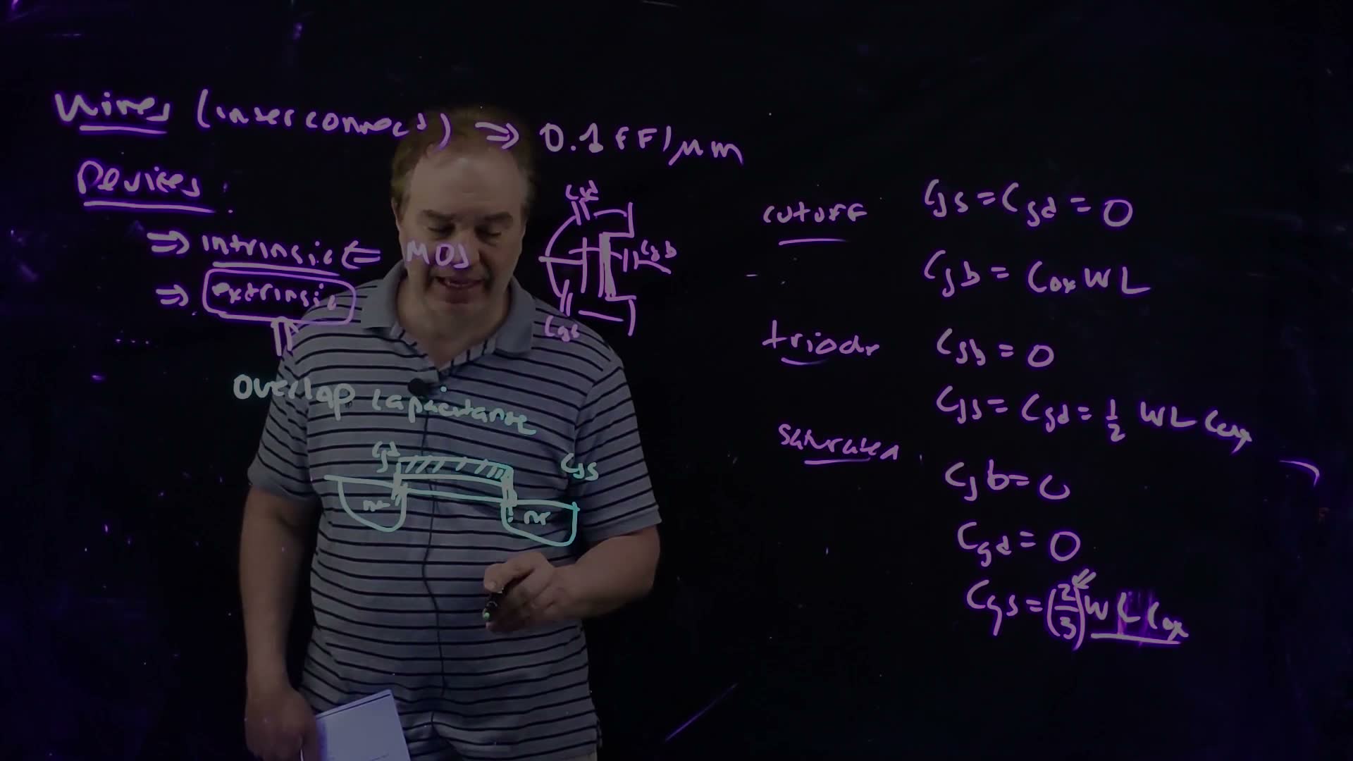
“Fundamentally digital integrated circuits work by charging and discharging capacitors with currents through transistors” (08:28). So there are two things to know: the current drive (Chapter 4) and the capacitance being charged. Wires also have resistance and inductance; those come later in the course (09:00). The capacitance comes from two places (09:23):

• wires, the interconnect;
• devices, the transistors themselves.

A wire’s capacitance depends on its surroundings, its width and much else. But a good rule of thumb for a minimum-width wire, which has held for several technology generations, is (09:27–10:00):

Wire capacitance, rule of thumbboard

$$C_{wire} \approx 0.1\ \mathrm{fF/\mu m}$$

Holds when: an average minimum-width wire; an estimate, not an extraction

Worked example. added A 100 µm wire has about $100 \times 0.1 = 10\,\mathrm{fF}$10fF. The chapter’s transistor has a gate capacitance of $1.60\,\mathrm{fF}$ (Section 3), so this short wire loads a gate like six transistor gates.

3. Intrinsic capacitance: the MOS capacitor by region

The idea. The oxide capacitance, $C_{ox}WL$Cox​WL, is what makes a MOSFET work, so it can never be removed. Where its other plate connects (to the body, or to the source and drain through the channel) depends on the region of operation.

The lecture splits a transistor’s capacitance into two kinds (10:27):

• intrinsic: the MOS capacitor itself, $C_{ox}$Cox​. “If you didn’t have $C_{ox}$Cox​, you basically wouldn’t have an MOS device.” It is fundamental to how the device works;
• extrinsic: capacitance that is there only because of how transistors are built (Sections 4 and 5).

The intrinsic capacitance divides into three parts: gate-to-source $C_{gs}$Cgs​, gate-to-drain $C_{gd}$ and gate-to-body $C_{gb}$ (10:54). How it divides depends on the region (11:23). Write $C_0 = C_{ox}WL$ for the whole MOS capacitor added.

• Cutoff (11:44). No inversion layer, so nothing connects the gate’s charge to the source or drain. All of the capacitance is gate-to-body.
• Triode (12:12). A fairly uniform inversion layer runs from source to drain. It shields the body: field lines from the gate end on the inversion layer instead, so $C_{gb} \to 0$0. The source and drain share the MOS capacitor about equally.
• Saturation (12:45). The inversion layer narrows toward the drain end and pinches off (Chapter 4). $C_{gb}$ is still zero, $C_{gd}$ is very small, and nearly all the capacitance is gate-to-source.

Intrinsic capacitances by regionboard

Region	$C_{gs}$	$C_{gd}$	$C_{gb}$
cutoff	0	0	$C_{ox}WL$
triode	$\tfrac12 C_{ox}WL$	$\tfrac12 C_{ox}WL$	0
saturation	$\tfrac23 C_{ox}WL$	0	0

Holds when: rules of thumb; compact models track the bias dependence properly

The two-thirds. In the long-channel limit, a correction factor of about $\tfrac23$ appears in saturation (13:24). “For all intents and purposes, most people in their back of the envelope calculation do not consider this two-thirds factor”: they take all the MOS capacitance, $C_{ox}WL$Cox​WL, to sit between gate and source (13:38). The lecture does exactly that in Sections 10 and 11. When you need an accurate answer, use the compact models in a circuit simulator, which also keep charge conserved (13:51).

About cutoff. added The Fall 2026 class added a refinement: in cutoff the depletion region below the oxide acts as a second capacitor in series, so $C_{gb}$ is somewhat less than $C_{ox}WL$Cox​WL. The board’s value is the upper limit.

Worked example. added The chapter’s device.

1. $C_{ox} = 6.39\times10^{-7}\,\mathrm{F/cm^2}$10−7F/cm2. Since $1\,\mathrm{F/cm^2} = 10^{15}\,\mathrm{fF}/10^8\,\mu\mathrm{m^2}$1015fF/108μm2, that is $6.39\,\mathrm{fF/\mu m^2}$6.39fF/μm2.
2. $C_0 = C_{ox}WL = 6.39 \times 1 \times 0.25 = 1.60\,\mathrm{fF}$1.60fF.
3. Triode: $C_{gs} = C_{gd} = 0.80\,\mathrm{fF}$0.80fF. Saturation: $C_{gs} = \tfrac23 \times 1.60 = 1.07\,\mathrm{fF}$1.07fF, or $1.60\,\mathrm{fF}$ with the back-of-the-envelope rule.
4. Per micron of width that is $1.6\,\mathrm{fF/\mu m}$1.6fF/μm. The Fall 2026 class quoted about 1–2 fF/µm as a historical rule of thumb added.

Check yourself Why is C_gb zero in the triode region, although the gate still sits above the body?

The inversion layer sits between them. Field lines from the gate end on the electrons of the channel, which connect to the source and drain, so a change in gate voltage changes the channel charge, not the body’s. The channel shields the body.

4. Overlap capacitance

The idea. Any part of the gate that sits next to the source or drain, rather than over the channel, couples to it directly. In older processes that was a deliberate overlap; today it is mostly the tall gate next to tall contacts.

Lecture05 @ 20:53Extrinsic capacitance: ① overlap (planar overlap, then tall gate and contacts) and ② source–drain junctions.

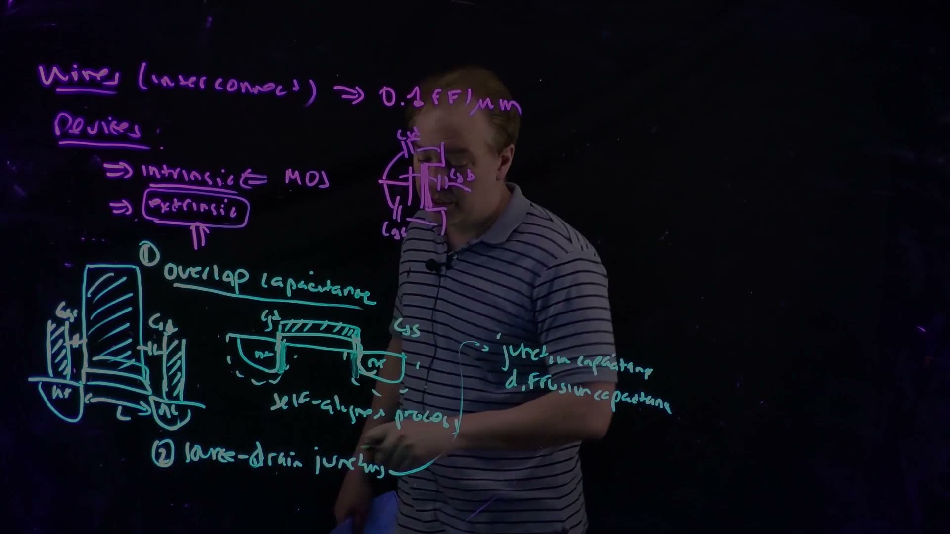
Extrinsic capacitance doesn’t help the device work; ideally it would all go away, “but unfortunately we’re stuck with it because of the way we build the transistors” (14:18). The first kind is overlap capacitance (14:47).

• In the old days (15:17), the inversion layer had to be sure to connect the source and the drain, so the gate was drawn slightly overlapping both. Each overlap is a small capacitor: gate-to-source and gate-to-drain.
• The self-aligned process (15:43–16:35) reduced it. The gate itself defines where the source and drain implants go, so the overlap regions become very small, and so does the overlap capacitance.
• In modern devices (16:35–17:56), a new capacitance acts just like it. To keep the gate’s resistance low while its length $L$ is tiny, gates are built very tall. The contacts to the source and drain are tall and skinny too. Side by side, the gate and those contacts form capacitors, gate-to-source and gate-to-drain, that look exactly like the “overlap capacitance of yesteryear”.

These depend on the layout, on where the contacts are placed. Usually they are lumped into the device models under assumptions about contact placement, and splitting them between the device models and parasitic extraction can get complicated (17:56).

5. Junction (diffusion) capacitance

The idea. The source and drain are reverse-biased pn junctions with the body, so each is a capacitor, $C_j = \kappa_s\varepsilon_0/W$ per area. Its value changes with the voltage across it.

The second extrinsic capacitance comes from the source and drain junctions (18:33). It is called junction capacitance, or diffusion capacitance, because the source and drain are “diffusions” (18:50).

A warning about the name (18:57–19:58). A forward-biased pn diode has a quite different “diffusion capacitance”, from the charge of minority carriers diffusing through it. This is not that. When this course says diffusion capacitance, it means the junction capacitance of the source and drain.

These junctions are always reverse-biased (or at zero bias), so their capacitance is exactly what Chapter 3 calculated (19:58); the problem set has you compute one. The lecture writes no new formula on the board. Restated from Chapter 3:

Junction capacitance (from Chapter 3)added

$$C_j = \frac{\kappa_s\varepsilon_0}{W}$$$$W = \sqrt{\frac{2\kappa_s\varepsilon_0\,(V_{bi} + V_R)}{qN}}$$

Holds when: reverse or zero bias; one-sided n+ junction, so N ≈ N_A of the body

The challenge: these capacitances are nonlinear (19:58). As the voltage across the junction changes, so does the capacitance, and it changes during circuit operation as the nodes switch (20:27).

reverse bias V_R (drain to body)

1.25 V

body doping N_A

10¹⁷ cm⁻³

drain area

0.50 µm²

built-in voltage V_bi

1.012 V

depletion width W

171 nm

C_j = κ_sε₀/W

0.605 fF/µm² (67% of its zero-bias value)

drain capacitance now

0.30 fF

as the drain swings 0 → 2.5 V

0.45 → 0.24 fF

The drain is an n⁺ region (N_D = 10²⁰ cm⁻³) in the p body, so nearly all the depletion width is on the body side and the body doping sets C_j. As the drain voltage rises the junction is reverse-biased harder, W grows as √(V_bi + V_R), and C_j falls: the capacitance changes during a switching event. Only the bottom area of the drain is counted.

What to notice.

• As the drain voltage rises from 0 to 2.5 V, the capacitance falls to about half.
• Lightly doped bodies give smaller junction capacitance: the depletion region is wider.
• The $n^+$ side is so heavily doped that it barely matters: the body sets $C_j$Cj​.

Worked example. added The chapter’s drain: $N_D = 10^{20}$ in a body of $N_A = 10^{17}\,\mathrm{cm^{-3}}$1017cm−3, with a bottom area of $1\,\mu\mathrm{m} \times 0.5\,\mu\mathrm{m}$0.5μm.

1. $V_{bi} = 0.02585\ln(10^{17}\cdot10^{20}/10^{20}) = 1.012\,\mathrm{V}$1.012V, and $N \approx N_A$NA​.
2. At $V_R = 0$0: $W = 114\,\mathrm{nm}$114nm, so $C_j = 1.036\times10^{-12}/1.14\times10^{-5} = 9.05\times10^{-8}\,\mathrm{F/cm^2} = 0.905\,\mathrm{fF/\mu m^2}$0.905fF/μm2.
3. At $V_R = 2.5\,\mathrm{V}$2.5V: $W = 213\,\mathrm{nm}$213nm, and $C_j = 0.486\,\mathrm{fF/\mu m^2}$0.486fF/μm2, 54% of the zero-bias value.
4. Over $0.5\,\mu\mathrm{m^2}$ the drain capacitance falls from $0.45$ to $0.24\,\mathrm{fF}$ as the drain rises from 0 to 2.5 V.
5. Compare the gate’s $1.60\,\mathrm{fF}$1.60fF: this bottom area alone gives $C_g/C_d$ of about 3.5 to 6.6. The overlap and contact capacitances of Section 4 add to the drain too, which is how real devices end up near the lecture’s $\eta \approx 1.5$–2 (Section 11).

Check yourself An inverter's output sits at 0 V. The NMOS body is at 0 V and the PMOS well at V_DD. Which drain junction has the larger capacitance per area, if both are doped alike?

The NMOS drain: it has zero bias across it, so its depletion region is narrowest and $C_j$ is largest. The PMOS drain is reverse-biased by the full $V_{DD}$VDD​. When the output swings to $V_{DD}$VDD​, the roles swap.

6. Sharing diffusions

The idea. Junction capacitance grows with junction area, and only capacitance on a switching node costs time. So a good layout merges diffusions, and puts the shared ones where they help.

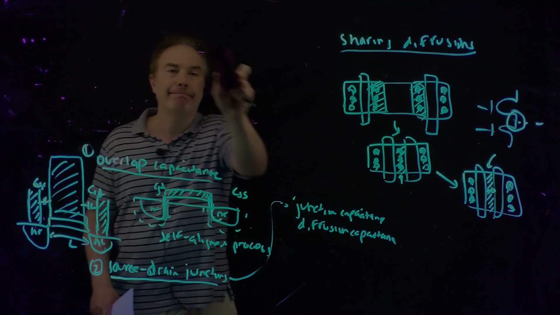
An important part of layout is keeping source and drain capacitance from slowing the circuit, by sharing diffusions (20:41). It came up in recitation too.

Lecture05 @ 23:40A series stack laid out three ways: separate devices, a shared contacted diffusion, and a shared uncontacted diffusion.

A series stack

Take two transistors in series, the source of one connected to the drain of the other (21:10). Three layouts:

1. Two separate transistors, each with its own contacted diffusions, joined by a metal wire (21:36). It works, but it is “a terrible decision”: the internal node carries the wire’s capacitance and two junction areas, and the layout takes more area (21:44–22:12).
2. One shared diffusion, still contacted (22:36). Less area and less junction capacitance.
3. A shared diffusion with no contacts (22:36). The internal node goes nowhere else, so it needs no contact. The design rules then let the two gates sit closer, and the junction shrinks further: the lowest capacitance on the internal node (23:06).

Two parallel transistors: a good and a poor choice

Lecture05 @ 26:47Two parallel NMOS (left), sharing the drain on C (centre) or the source on ground (right, 'poor choice').

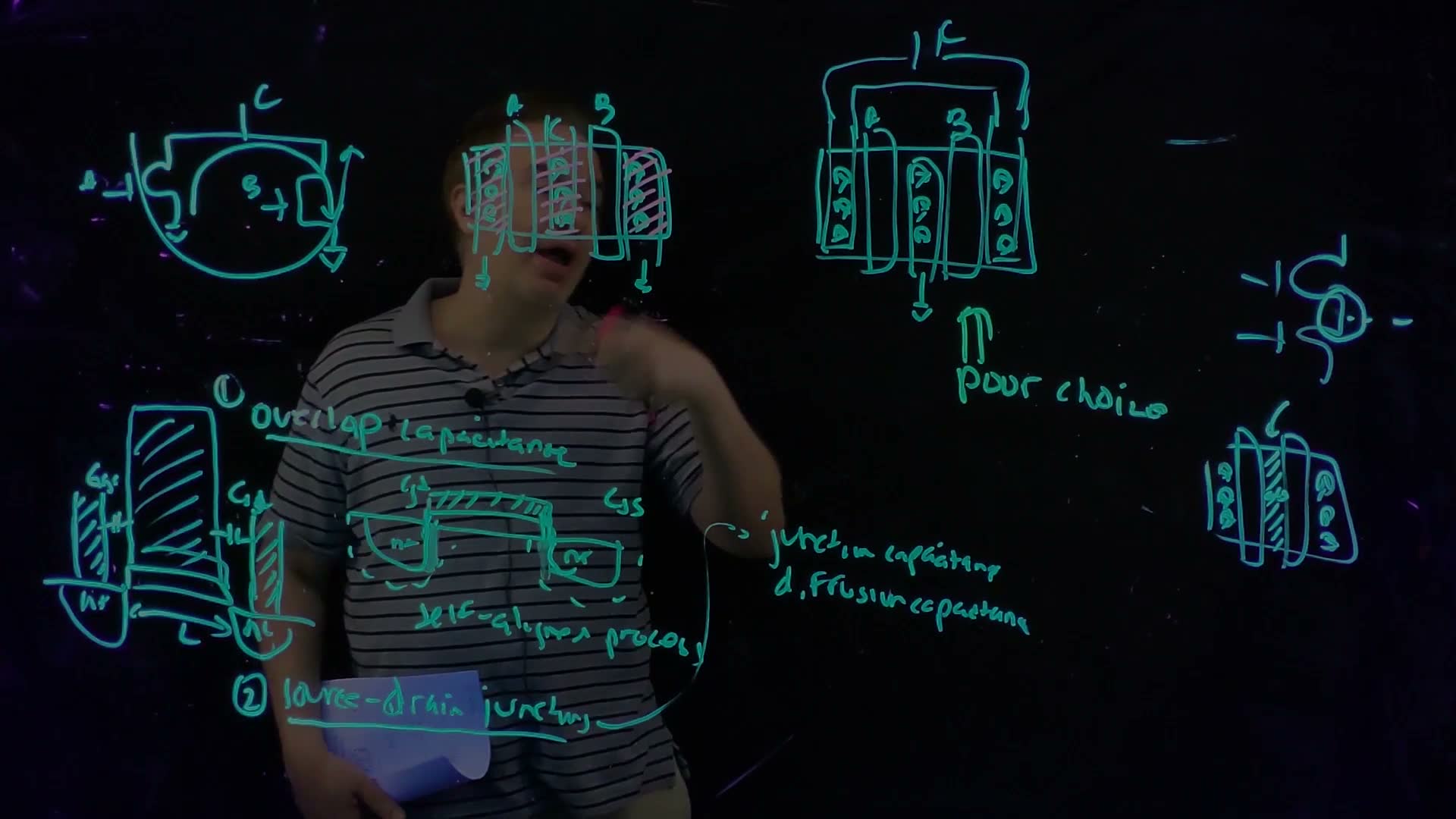
Now two transistors in parallel, gates A and B, both drains joined at the output node C, both sources at ground (23:44). There are two ways to share a diffusion (24:00–25:32):

• share the drains: the middle diffusion is node C, and the two outer diffusions go to ground;
• share the sources: the middle diffusion goes to ground, and the two outer diffusions are wired together to form C.

Before reading on, decide which is better. “If this were a normal class, this is one of those places where I would step back and say, okay, tell me which of these is the good one” (25:32).

The second is the poor choice (25:59). Count the junction areas on each node (26:07–27:08):

• sharing the drains puts one junction area on C and two on ground;
• sharing the sources puts one on ground and two on C.

“I don’t care about capacitance that’s tied to ground. I’m not switching it” (26:39). Capacitance on ground even helps: it is decoupling capacitance, which the course meets with power distribution. But C switches, so every junction area on C must be charged and discharged.

Worked example. added With equal diffusions of the chapter’s $0.45\,\mathrm{fF}$ each (zero bias, Section 5), sharing the drains puts $0.45\,\mathrm{fF}$ of junction capacitance on C; sharing the sources puts $0.90\,\mathrm{fF}$0.90fF, plus the wire joining the two outer diffusions.

Both layouts are correct circuits. added A layout-versus-schematic (LVS) check passes either one. It checks connections, not capacitance, so a poor choice won’t be caught there (a Fall 2026 class addition).

Check yourself A NAND gate's two series NMOS share an internal node that connects nowhere else. Why can the shared diffusion go without a contact, and what does that buy?

Nothing outside needs to reach the internal node, so it needs no contact. Without one, the design rules let the two gates sit closer together, which shrinks the shared junction: less area and less capacitance on that internal node (23:06).

7. The inverter’s load: gate and drain capacitance

The idea. When one inverter drives another, its output node carries its own drain junctions plus the next inverter’s gates. For estimates, these are lumped into a drain capacitance $C_d$ and a gate capacitance $C_g$Cg​.

Lecture05 @ 29:41An inverter driving an inverter: drain–body capacitances at the output, gate–source capacitances of the load.

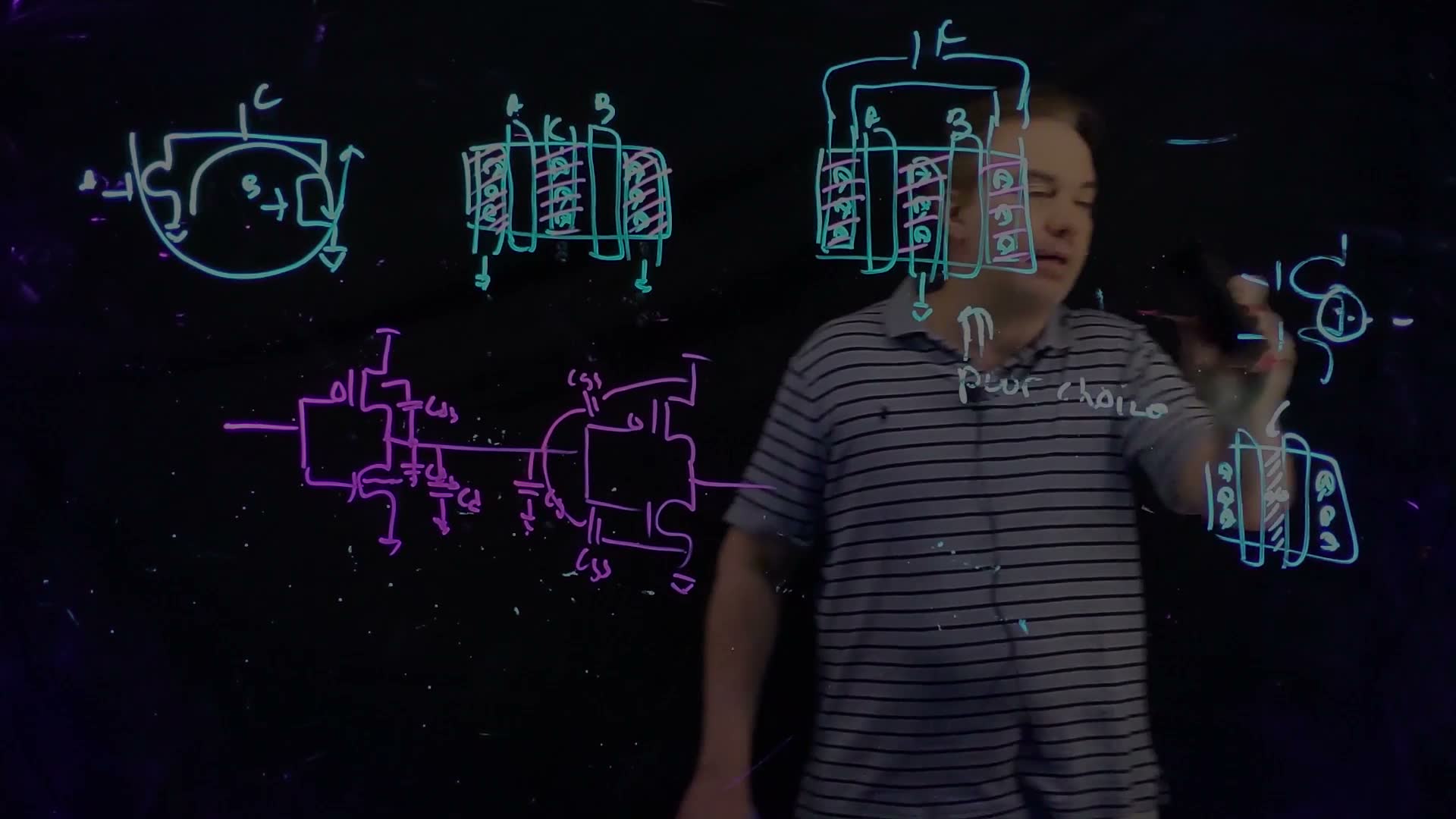
The CMOS inverter, an NFET and a PFET with joined gates and joined drains, is “the quintessential CMOS digital circuit”; the next lecture covers it in detail (27:34). Here only its capacitances matter (28:01–29:20):

• at the driver’s output, the capacitance is dominated by the two drain-to-body (junction) capacitances, of the NFET and of the PFET;
• the inverter being driven presents mainly the gate-to-source capacitances of its two transistors.

For back-of-the-envelope analysis these are lumped together (29:07): the driving gate has an equivalent drain capacitance $C_d$ at its output, and it drives an equivalent gate capacitance $C_g$Cg​. Sections 11–13 use exactly these two numbers.

8. Wells and body connections

The idea. NFETs sit in the p substrate and PFETs in an n well. Tying the substrate to ground and the well to $V_{DD}$ keeps every junction reverse-biased, whatever the circuit does.

Lecture05 @ 33:52NFET in the p substrate, PFET in an n well, with body taps to ground and V_DD; 'triple well'.

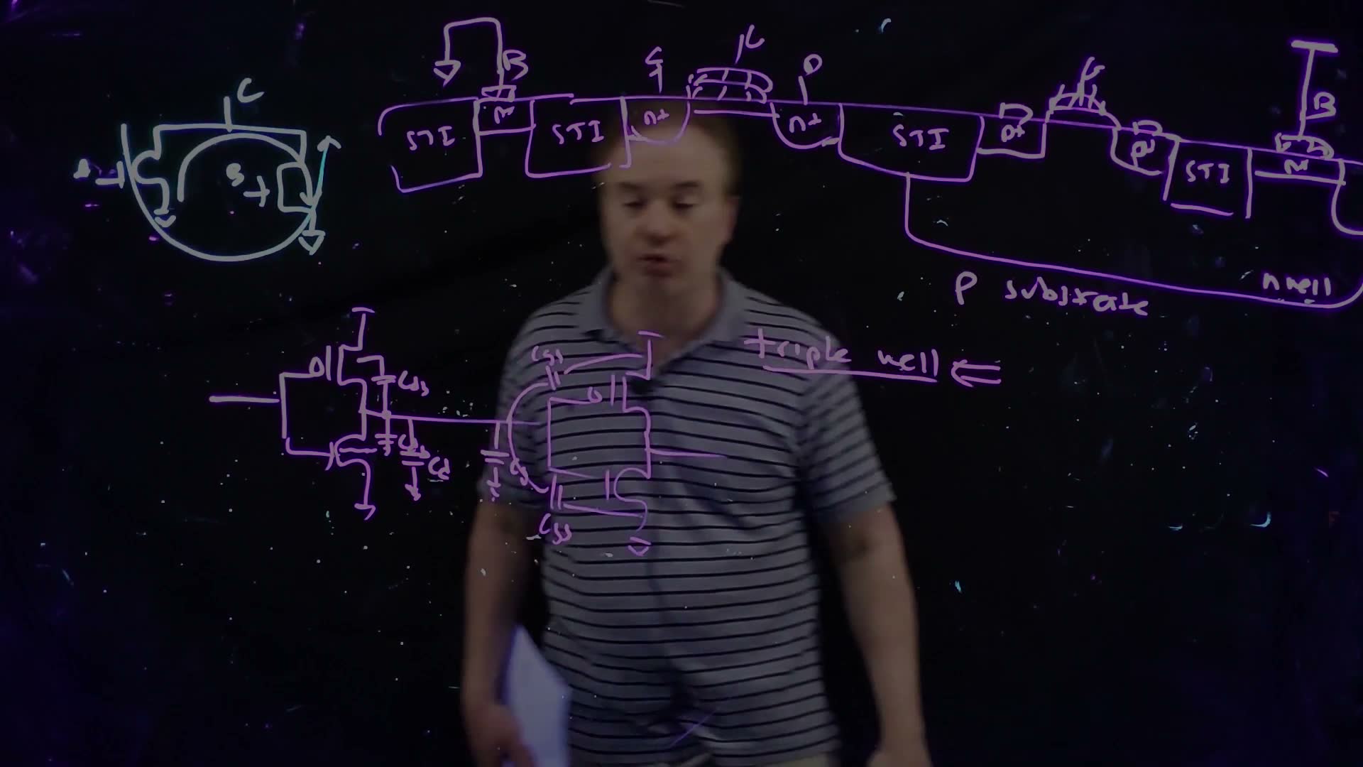
The basics of how PFETs and NFETs are combined (29:34–31:33):

• on a p-type substrate, NFETs are built directly in the substrate, between regions of shallow trench isolation (STI, Chapter 3);
• the substrate gets a $p^+$ contact, the plug to the body, which many transistors can share;
• PFETs need an n-type body, so they are built in an n well, which has its own $n^+$ well contact.

Tie the well to $V_{DD}$ and the substrate to ground (31:33). Then (32:00–33:09):

• the n-well/p-substrate junction is always reverse-biased, by the full $V_{DD}$VDD​;
• no PFET source or drain can rise above the well, so their junctions can never be forward-biased;
• no NFET source or drain can fall below the substrate, so theirs can’t either.

That matters: if a junction becomes forward-biased, “these circuits just don’t work anymore”. If a design ties a body anywhere else, you have to check that this can’t happen (32:58).

Triple well (33:09–33:48). Some technologies nest one more level: an NFET in a p well inside an n well inside the p substrate. That gives NFETs bodies that can be controlled independently, or more isolation from the substrate.

Check yourself Why tie the n well to the highest voltage in the circuit rather than to, say, V_DD/2?

The PMOS sources and drains are p-type regions in the n well. If any of them could go above the well’s voltage, that junction would be forward-biased and conduct. With the well at the highest voltage, that can never happen.

Check yourself An inverter's PFET has its n well tied to ground instead of V_DD. With V_DD = 2.5 V and V_in = 0, does static DC current flow?

Yes, a large one. Look at the device’s structure, not only its symbol. The PFET’s $p^+$ source sits at $V_{DD} = 2.5\,\mathrm{V}$ inside an n well at 0 V, so that $p^+$/n junction is forward-biased by 2.5 V. Current flows from $V_{DD}$ through the source junction into the well and out through the well contact to ground, whatever the transistors are doing. In the Fall 2026 class the instructor called a circuit with a forward-biased junction “a classic exam problem that I often give” (its Lecture 4, 30:09). (This is MT17-1b.)

9. Figures of merit and the small-signal model

The idea. To compare transistors, engineers quote one-number figures of merit. The lecture’s is $f_T$fT​, found from a small-signal model with just a gate capacitance and a controlled current source.

Lecture05 @ 37:03Figures of merit: f_T, the unity-gain cut-off frequency, and the small-signal model.

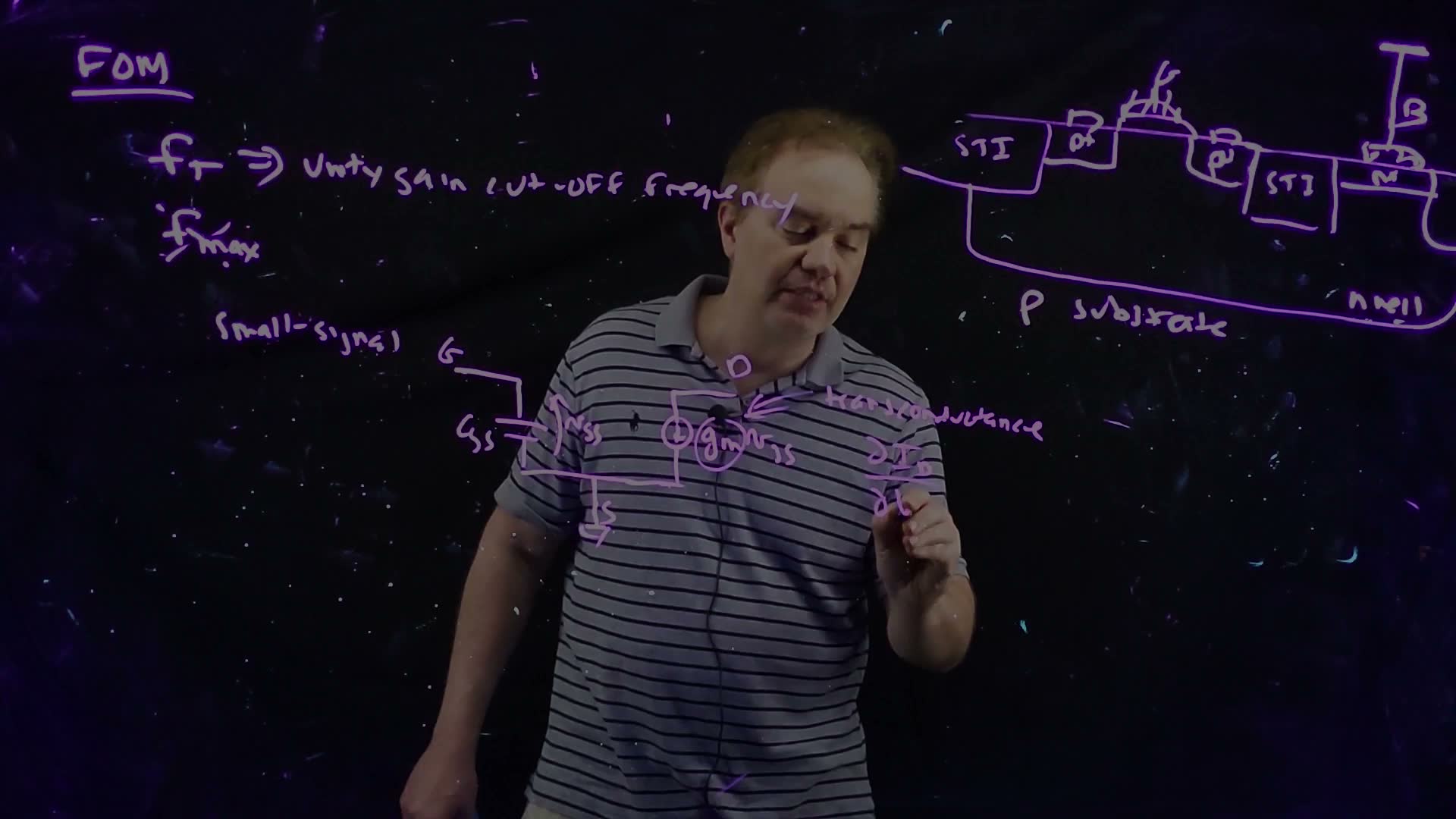
A figure of merit combines parameters into one number that lets you compare a design with the alternatives (34:32). For devices, two common ones let you say “my device is faster than your device”: $f_T$ and $f_{max}$fmax​, both frequencies (35:01). The lecture covers only $f_T$fT​, the unity-gain cut-off frequency (35:28).

To define it, use a small-signal model (35:47–37:10):

• choose an operating point with the device saturated, in a common-source configuration: source grounded;
• between gate and source, a capacitor $C_{gs}$Cgs​, with the small-signal voltage $v_{gs}$ across it;
• between drain and source, a current source $g_m v_{gs}$gm​vgs​.

Transconductanceboard

$$g_m = \left.\frac{\partial I_D}{\partial V_{GS}}\right|_{V_{DS}}$$

How much the drain current changes per volt of gate-source voltage, in A/V (siemens).

Holds when: small signals about a saturated operating point

10. The unity-gain frequency and the transit time

The idea. At high frequency, the gate current needed to charge $C_{gs}$ grows, while the drain current it controls doesn’t. The frequency at which the two are equal is $f_T = g_m/(2\pi C_{gs})$gm​/(2πCgs​), and it comes out as one over $2\pi$ times the time carriers take to cross the channel.

Lecture05 @ 42:35f_T: the current gain i_d/i_g (bottom), ω_T and f_T (right), and f_T = v_sat/(2πL) = 1/(2πτ_tr) (top).

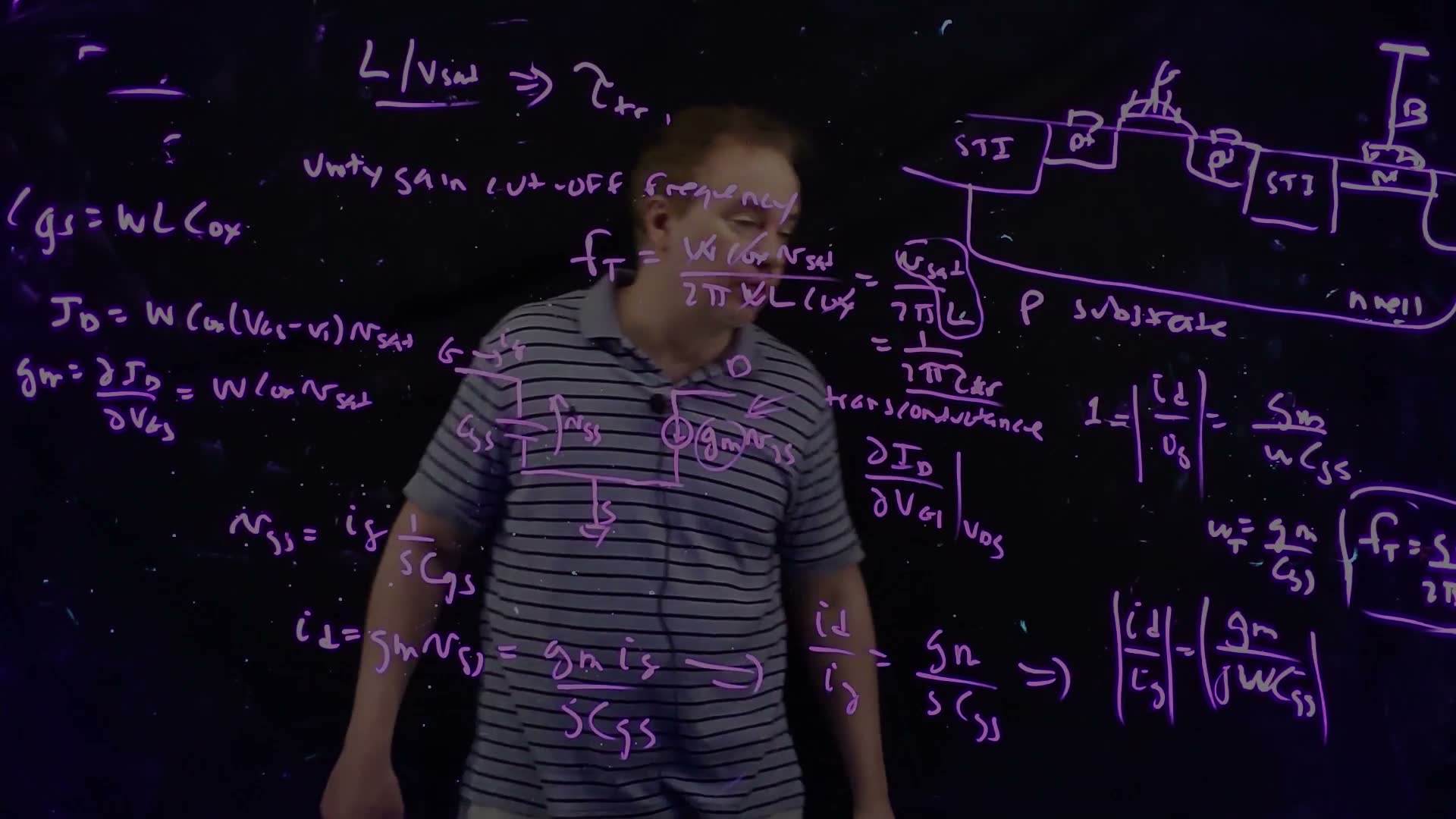
The current gain

Drive the gate with a small current $i_g$ and short the drain, so $i_d$ is the output current. Work in the Laplace domain (37:14):

Unity-gain frequency (board, 37:14–39:33)

1. The gate current flows into $C_{gs}$ board: $v_{gs} = i_g\cdot\dfrac{1}{sC_{gs}}$sCgs​1​.
2. The drain current is set by $v_{gs}$ board: $i_d = g_m v_{gs} = \dfrac{g_m i_g}{sC_{gs}}$sCgs​gm​ig​​.
3. The current gain board: $\dfrac{i_d}{i_g} = \dfrac{g_m}{sC_{gs}}$sCgs​gm​​.
4. Go to sinusoids, $s = j\omega$jω, and take the magnitude board: $\left|\dfrac{i_d}{i_g}\right| = \dfrac{g_m}{\omega C_{gs}}$ωCgs​gm​​, since $|j| = 1$1.
5. The gain falls as $1/\omega$1/ω. Set it to 1 and solve board: $\omega_T = \dfrac{g_m}{C_{gs}}$Cgs​gm​​, in rad/s.
6. Divide by $2\pi$ for hertz board: $f_T = \dfrac{g_m}{2\pi C_{gs}}$2πCgs​gm​​.

At 37:25 the speech calls $i_g$ “the small signal drain current”; the board draws it flowing into the gate. It is the gate current.

In terms of the device

“I can take this one step further, which I think is very interesting” (39:39). Use the lecture’s simple device expressions (39:52–41:07):

The unity-gain frequency from the device (board, 39:52–41:07)

1. Take all of the MOS capacitance as gate-to-source (Section 3) board: $C_{gs} = WLC_{ox}$WLCox​.
2. Take the velocity-saturated current (Chapter 4) board: $I_D = WC_{ox}(V_{GS} - V_T)\,v_{sat}$VT​)vsat​.
3. Differentiate with respect to $V_{GS}$ board: $g_m = WC_{ox}v_{sat}$WCox​vsat​.
4. Substitute board: $f_T = \dfrac{WC_{ox}v_{sat}}{2\pi\,WLC_{ox}}$2πWLCox​WCox​vsat​​. The $W$ and the $C_{ox}$ cancel.
5. What’s left board: $f_T = \dfrac{v_{sat}}{2\pi L}$2πLvsat​​.

The transit time

What is $L/v_{sat}$ (41:21)? Its units are cm ÷ (cm/s) = s, a time. $L$ is the channel length and $v_{sat}$ is the speed of the carriers crossing it, so $L/v_{sat}$ is how long a carrier takes to get from source to drain: the transit time (41:56).

Unity-gain frequency and transit timeboard

$$f_T = \frac{g_m}{2\pi C_{gs}} = \frac{v_{sat}}{2\pi L}$$$$\tau_{tr} = \frac{L}{v_{sat}}, \qquad f_T = \frac{1}{2\pi\tau_{tr}}$$

Holds when: saturated, fully velocity-saturated device; C_gs = WLC_ox; the small-signal model of Section 9

“Which is very cool” (42:14). A small-signal property of the device, $f_T$fT​, comes straight from a physical picture: carriers crossing the channel. It also says why shrinking the channel makes the device faster: carriers at the same velocity cross a shorter distance in less time.

Worked example. added The chapter’s device.

1. $g_m = WC_{ox}v_{sat} = 10^{-4} \times 6.39\times10^{-7} \times 10^7 = 6.39\times10^{-4}\,\mathrm{A/V} = 0.639\,\mathrm{mS}$0.639mS.
2. $C_{gs} = WLC_{ox} = 1.60\,\mathrm{fF}$ (Section 3).
3. $f_T = 6.39\times10^{-4}/(2\pi \times 1.60\times10^{-15}) = 63.7\,\mathrm{GHz}$63.7GHz.
4. Directly: $\tau_{tr} = L/v_{sat} = 2.5\times10^{-5}/10^7 = 2.5\times10^{-12}\,\mathrm{s} = 2.5\,\mathrm{ps}$2.5ps, and $1/(2\pi \times 2.5\,\mathrm{ps}) = 63.7\,\mathrm{GHz}$63.7GHz. The two routes agree.

How good is the estimate? added $g_m = WC_{ox}v_{sat}$ is the slope of the fully velocity-saturated current. Chapter 4 found that at 0.25 µm this device reaches only about half of that limiting current (0.591 mA against 1.28 mA), so its real $g_m$ is lower, and $f_T = v_{sat}/(2\pi L)$ is an optimistic, upper estimate. It is the right scale and the right trend: $f_T \propto 1/L$1/L.

Common mistakes.

• Expecting a wider transistor to have a higher $f_T$fT​. Width raises $g_m$ and $C_{gs}$ together, and it cancels.
• Mixing the two choices for $C_{gs}$Cgs​. With $\tfrac23 WLC_{ox}$32​WLCox​, $f_T$ would be 1.5 times higher (95.5 GHz here). The lecture’s $f_T = v_{sat}/(2\pi L)$ uses $C_{gs} = WLC_{ox}$WLCox​.

Check yourself The channel length is halved, with v_sat unchanged. What happens to τ_tr and f_T? And if W is doubled instead?

Halving $L$ halves $\tau_{tr} = L/v_{sat}$ and doubles $f_T$fT​. Doubling $W$ doubles both $g_m$ and $C_{gs}$Cgs​, so $f_T$ doesn’t change.

11. From the unity-gain frequency to switching delay

The idea. The time for one transistor to discharge another’s gate is the charge divided by the current. With the lecture’s simple models, that time is the transit time times a factor that counts the drain capacitance.

$f_T$ is a small-signal, “analogish” quantity (42:47). How does it relate to large-signal digital switching? The lecture builds the link in steps.

Digital figures of merit: FO1 and FO4

There are figures of merit for switching too (44:00). Two are common, both defined with CMOS inverters (44:24–45:46):

• the fan-out-of-one delay, FO1: the delay of an inverter driving one inverter of exactly its own size;
• the fan-out-of-four delay, FO4: the delay of an inverter driving four inverters of its own size.

In a good design most gates are loaded about like FO4, so FO4 is a good measure of the average gate delay in a microprocessor (45:46). Designers count “the number of fan-out-of-fours between my flip-flops”, and that sets the clock frequency (45:57).

The chain of reasoning the lecture is after (46:30): from $L$ and $v_{sat}$vsat​, estimate $f_T$fT​; from $f_T$fT​, the FO1 and FO4; from FO4 and the pipeline depth, the clock frequency. “You can start with very little information and … get pretty close to the right answer.”

Lecture05 @ 53:29One NFET discharging an equal NFET: t ≅ V_DD(C_g + C_d)/I_Dsat = τ_tr(1 + 1/η).

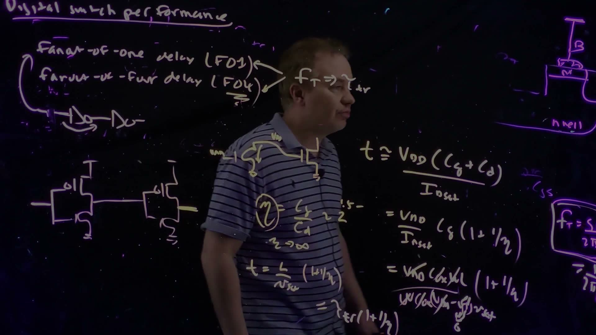
One NFET discharging another

Start with just NFETs (46:58). One NFET discharges the gate of another NFET of the same size, which starts charged to $V_{DD}$ (47:24). Flip the first one’s gate quickly from 0 to $V_{DD}$VDD​; it moves quickly into saturation, so its saturated current $I_{DSAT}$ does the discharging (47:59).

The time is the charge to remove divided by the current. The charge is the voltage times the capacitance on this node: the gate capacitance $C_g$ of the second device plus the drain capacitance $C_d$ of the first (47:49).

Carry the drain capacitance along as a ratio (48:35):

$$\eta = \frac{C_g}{C_d} .$$

Ideally $\eta$ would be infinite: no drain capacitance at all. In reality it is about 1.5 to 2, “unfortunately” (48:35).

NFET-to-NFET delay (board, 47:24–50:24)

1. Charge over current board: $t \approx \dfrac{V_{DD}(C_g + C_d)}{I_{DSAT}}$IDSAT​VDD​(Cg​+Cd​)​.
2. Bring in $\eta$η, so $C_d = C_g/\eta$ board: $t = \dfrac{V_{DD}}{I_{DSAT}}\,C_g\left(1 + \dfrac{1}{\eta}\right)$IDSAT​VDD​​Cg​(1+η1​).
3. Substitute $C_g = C_{ox}WL$ and the velocity-saturated $I_{DSAT} = WC_{ox}(V_{DD} - V_T)v_{sat}$ board: $t = \dfrac{V_{DD}\,C_{ox}WL}{WC_{ox}(V_{DD} - V_T)\,v_{sat}}\left(1 + \dfrac{1}{\eta}\right)$WCox​(VDD​−VT​)vsat​VDD​Cox​WL​(1+η1​).
4. Assume $V_{DD} \gg V_T$ and drop $V_T$ board. Then $V_{DD}$VDD​, $W$ and $C_{ox}$ cancel: $t = \dfrac{L}{v_{sat}}\left(1 + \dfrac{1}{\eta}\right)$vsat​L​(1+η1​).
5. And $L/v_{sat}$ is the transit time again board: $t = \tau_{tr}\left(1 + \dfrac{1}{\eta}\right)$τtr​(1+η1​).

“Isn’t that nice?” (50:34). Since $f_T = 1/(2\pi\tau_{tr})$1/(2πτtr​), knowing $f_T$ gives $\tau_{tr}$τtr​, and $\tau_{tr}$ gives this delay.

Worked example. added The chapter’s device, with $\eta = 2$2.

1. $t = \tau_{tr}(1 + 1/\eta) = 2.5 \times 1.5 = 3.75\,\mathrm{ps}$3.75ps.
2. Keeping $V_T$ instead of dropping it multiplies this by $V_{DD}/(V_{DD} - V_T) = 2.5/2.0 = 1.25$1.25: $4.69\,\mathrm{ps}$ (the Fall 2026 class kept this factor).
3. With Chapter 4’s full velocity-saturated current instead, $I_{DSAT} = 0.591\,\mathrm{mA}$0.591mA, step 1 of the derivation gives $t = 2.5 \times (1.60 + 0.80)\,\mathrm{fF}/0.591\,\mathrm{mA} = 10.1\,\mathrm{ps}$10.1ps, 2.7 times longer. The transit-time formula is the quick, optimistic version.

12. The fan-out-of-one delay

The idea. In an inverter, the PFET is made twice as wide to match the NFET’s current, so it brings twice the gate and drain capacitance. That makes the inverter’s FO1 three times the single-NFET delay.

Lecture05 @ 60:10FO1 = 3τ_tr(1 + 1/η) (bottom), and FO4 = ((4C_g + C_d)/(C_g + C_d)) FO1 = (1 + 4η)(3/η)τ_tr (right).

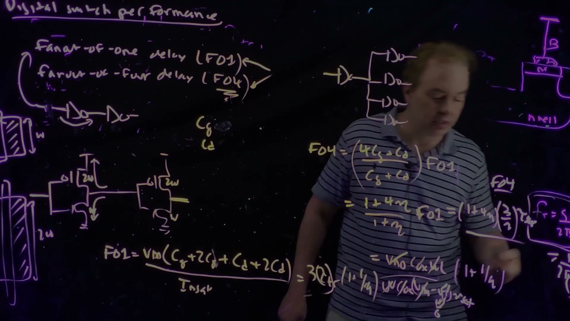
Sizing the PFET

Size the inverter so that, at the same overdrive, the PFET and the NFET give the same current (51:32). A PFET’s carriers are holes, whose saturation velocity is about half that of electrons (Chapter 4). With $I_{DSAT} = WC_{ox}v_{sat}(V_{GS} - V_T)$VT​), half the velocity needs twice the width: NFET $W$W, PFET $2W$ (53:17).

The lecture adds a caveat (52:00–53:48):

• long channels: going by mobility alone, PFETs were about 3× worse;
• velocity saturated: about 2× worse, the factor used here, and true through about the 22 nm node;
• modern FinFET technologies: strain engineering, including germanium in the channel, has brought holes and electrons to about the same source injection velocity (Chapter 4). PFETs and NFETs now drive about the same current. “Always buyer beware on that point.”

Counting the capacitance

Now an inverter drives one identical inverter (53:48–55:26). The output node carries:

• the load inverter’s gate capacitance: the NFET’s $C_g$Cg​, and the PFET’s $2C_g$2Cg​, since it is twice as wide;
• the driver’s drain capacitance: the NFET’s $C_d$Cd​, and the PFET’s $2C_d$2Cd​, since a $2W$ device has twice the junction area (55:09).

Discharging through the NFET (or charging through the PFET, which gives the same current by design) (55:26):

FO1 (board, 53:48–56:11)

1. Charge over current board: $\mathrm{FO1} = \dfrac{V_{DD}(C_g + 2C_g + C_d + 2C_d)}{I_{DSAT}} = \dfrac{3V_{DD}(C_g + C_d)}{I_{DSAT}}$IDSAT​3VDD​(Cg​+Cd​)​.
2. That is three times the NFET-to-NFET delay of Section 11, step 1 added.
3. So board: $\mathrm{FO1} = 3\tau_{tr}\left(1 + \dfrac{1}{\eta}\right)$3τtr​(1+η1​).

Worked example. added With $\tau_{tr} = 2.5\,\mathrm{ps}$ and $\eta = 2$2: $\mathrm{FO1} = 3 \times 2.5 \times 1.5 = 11.25\,\mathrm{ps}$11.25ps.

Check yourself Why does the 2W PFET triple the load rather than double it?

The load is the NFET’s capacitance plus the PFET’s. The PFET is twice as wide, so it has twice the gate capacitance and twice the drain junction area: $C + 2C = 3C$3C, for both the gate and the drain parts.

13. The fan-out-of-four delay

The idea. Four loads multiply the gate capacitance by four, but the driver still has only its own one drain capacitance. So FO4 is less than four times FO1.

“Your first knee-jerk reaction would be, well, fan-out of four is gonna be four times fan-out of one” (56:57). It isn’t. Four times FO1 would also count four drain capacitances, but there is still only one driver, with one drain (57:24). The gate load goes up by four; the drain load doesn’t.

The lecture changes notation here, and apologises for it (57:40–58:07): from now on $C_G$ and $C_D$ mean the gate and drain capacitance of the whole inverter, three times the NFET’s. Their ratio is still $\eta$η.

FO4 (board, 57:40–59:42)

1. FO1 drives $C_G + C_D$CD​; FO4 drives $4C_G + C_D$ with the same current. Divide FO1 by $C_G + C_D$ and multiply by $4C_G + C_D$ board: $\mathrm{FO4} = \dfrac{4C_G + C_D}{C_G + C_D}\,\mathrm{FO1}$CG​+CD​4CG​+CD​​FO1.
2. Check the limit (58:53): with no drain capacitance, $C_D \to 0$0, the ratio is $4C_G/C_G = 4$4, and only then is FO4 four times FO1.
3. Divide top and bottom by $C_D$ and use $\eta = C_G/C_D$ board: $\mathrm{FO4} = \dfrac{1 + 4\eta}{1 + \eta}\,\mathrm{FO1}$1+η1+4η​FO1.
4. Substitute $\mathrm{FO1} = 3\tau_{tr}(1 + \eta)/\eta$ board: $\mathrm{FO4} = (1 + 4\eta)\dfrac{3}{\eta}\,\tau_{tr}$4η)η3​τtr​.

At 58:30 the speech says “divide it by $C_G$ minus $C_D$CD​”; the board adds, $C_G + C_D$CD​, as it must: FO1’s load is the sum.

Transit-time delay estimatesboard

$$t_{\text{NFET}} = \tau_{tr}\left(1 + \frac{1}{\eta}\right)$$$$\mathrm{FO1} = 3\tau_{tr}\left(1 + \frac{1}{\eta}\right)$$$$\mathrm{FO4} = \frac{1 + 4\eta}{1 + \eta}\,\mathrm{FO1} = (1 + 4\eta)\frac{3}{\eta}\,\tau_{tr}$$

added The same FO4 in another form is $3\tau_{tr}(4 + 1/\eta)$1/η).

Holds when: velocity-saturated devices with V_DD ≫ V_T; PFET 2W for equal drive; η = C_g/C_d; wires ignored

The whole chain (59:46). From the transit time (or $f_T$fT​) to FO4, and from FO4 and the pipeline depth to the clock rate. It also shows why Dennard scaling (Chapter 4) made chips faster: a shorter channel means a shorter transit time, and every delay above shrinks with it.

channel length L (v_sat = 10⁷ cm/s)

0.25 µm

η = C_g/C_d

2.0

fan-out N

4

transit time τ_tr = L/v_sat

2.50 ps

f_T = 1/(2πτ_tr)

63.7 GHz

one NFET into an equal NFET, τ_tr(1 + 1/η)

3.75 ps

FO1 = 3τ_tr(1 + 1/η)

11.25 ps

FO4 = 3τ_tr(4 + 1/η)

33.75 ps = 3.00 × FO1, not 4 ×

Each extra receiving inverter adds the same gate load, so the delay grows in equal steps of 3τ_tr. The driver's own drain capacitance is paid once, which is why the line starts above zero and FO4 is less than four times FO1. Raise η (less drain capacitance) and the two lines come together. The lecture works out N = 1 and N = 4; the other points use the same counting.

What to notice.

• Each extra load adds the same $3\tau_{tr}$3τtr​: the line is straight, but it doesn’t start at zero. The offset is the driver’s own drain capacitance.
• With $\eta = 2$2, FO4 is 3.0 times FO1, not 4. As $\eta$ grows the drain matters less and the ratio approaches 4.
• Shortening $L$ scales every delay down together, and raises $f_T$fT​.

Worked example. added The chapter’s device, $\tau_{tr} = 2.5\,\mathrm{ps}$2.5ps.

1. $\eta = 2$2: $\mathrm{FO4} = \dfrac{1 + 8}{1 + 2} \times 11.25 = 3 \times 11.25 = 33.75\,\mathrm{ps}$33.75ps. Four times FO1 would give 45 ps, a third too much.
2. Check with the other form: $(1 + 8)(3/2)(2.5) = 33.75\,\mathrm{ps}$33.75ps.
3. $\eta = 1.5$1.5: the ratio is $(1 + 6)/(1 + 1.5) = 2.8$2.8.
4. A clock cycle of 20 FO4 would last $20 \times 33.75 = 675\,\mathrm{ps}$675ps, a clock of $1/675\,\mathrm{ps} = 1.48\,\mathrm{GHz}$1.48GHz. The count of 20 is only for illustration; it depends on the design.

Common mistakes.

• Multiplying FO1 by four. Only the gate load scales with the fan-out.
• Forgetting the change of notation at 57:40: in the FO4 formula, $C_G$ and $C_D$ belong to the whole inverter. Since both are three times the NFET’s, $\eta$ is unchanged.
• Treating these as accurate delays. They neglect $V_T$VT​, wires and the details of the switching waveform, and they use the fully velocity-saturated current.

Check yourself A technology has η = 1. What are FO1 and FO4 in units of τ_tr, and what is FO4/FO1?

$\mathrm{FO1} = 3\tau_{tr}(1 + 1) = 6\tau_{tr}$6τtr​. $\mathrm{FO4} = (1 + 4)(3/1)\tau_{tr} = 15\tau_{tr}$15τtr​. The ratio is $(1 + 4)/(1 + 1) = 2.5$2.5.

Check yourself Suppose the PFET drives exactly the same current as an NFET of the same width, so the inverter is W/W. What are FO1 and FO4 in terms of τ_tr and η?

Count the capacitance again with a $W$ PFET. FO1’s load is $C_g + C_g$ of gate and $C_d + C_d$ of drain, and the NFET’s current discharges it:

$$\mathrm{FO1} = \frac{V_{DD}(2C_g + 2C_d)}{I_{DSAT}}$$

As in Section 11, $V_{DD}C_g/I_{DSAT} = \tau_{tr}$ and $C_d = C_g/\eta$Cg​/η, so

$$\mathrm{FO1} = 2\tau_{tr}\left(1 + \frac{1}{\eta}\right) .$$

FO4 has four loads’ gates but one driver’s drains, $8C_g + 2C_d$2Cd​:

$$\mathrm{FO4} = 2\tau_{tr}\left(4 + \frac{1}{\eta}\right) .$$

The factor 3 of the 2W/W inverter becomes 2, and the ratio $\mathrm{FO4}/\mathrm{FO1} = (1 + 4\eta)/(1 + \eta)$ is unchanged. With $\tau_{tr} = 2.5\,\mathrm{ps}$ and $\eta = 2$2: FO1 = 7.5 ps and FO4 = 22.5 ps. (This is MT21-2.)

Formulas to remember

Formula	Meaning
$V_T = V_{FB} + 2\phi_F + Q_{bulk}/C_{ox}$Qbulk​/Cox​, $Q_{bulk} = \sqrt{2qN_A\kappa_s\varepsilon_0(2\phi_F + V_{SB})}$	body effect: $V_T$ rises with $V_{SB}$
$C_{wire} \approx 0.1$ fF/µm	minimum-width wire, rule of thumb
cutoff $C_{gb} = C_{ox}WL$Cox​WL; triode $C_{gs} = C_{gd} = \tfrac12 C_{ox}WL$21​Cox​WL; saturation $C_{gs} = \tfrac23 C_{ox}WL$ (often $C_{ox}WL$Cox​WL)	intrinsic capacitance by region
$C_j = \kappa_s\varepsilon_0/W$κs​ε0​/W, falls with reverse bias	junction (diffusion) capacitance
share drains on the switching node; well to $V_{DD}$VDD​, substrate to ground	layout and body connections
$g_m = \partial I_D/\partial V_{GS}$∂ID​/∂VGS​; $g_m = WC_{ox}v_{sat}$ (velocity saturated)	transconductance
$f_T = g_m/(2\pi C_{gs}) = v_{sat}/(2\pi L) = 1/(2\pi\tau_{tr})$1/(2πτtr​), $\tau_{tr} = L/v_{sat}$	unity-gain frequency, transit time
$t \approx V_{DD}(C_g + C_d)/I_{DSAT} = \tau_{tr}(1 + 1/\eta)$1/η), $\eta = C_g/C_d \approx 1.5$–2	NFET discharging an equal NFET
$\mathrm{FO1} = 3\tau_{tr}(1 + 1/\eta)$	PFET $2W$ triples the load
$\mathrm{FO4} = \dfrac{1 + 4\eta}{1 + \eta}\mathrm{FO1} = (1 + 4\eta)\dfrac{3}{\eta}\tau_{tr}$	not $4\times$FO1

The lecture’s boards

Lecture05 @ 08:09 body effect: Q_bulk with V_SB

Lecture05 @ 15:49 wires; intrinsic capacitance by region

Lecture05 @ 20:53 overlap and junction capacitance

Lecture05 @ 23:40 sharing diffusions in a stack

Lecture05 @ 26:47 parallel NMOS: the poor choice

Lecture05 @ 29:41 inverter load: C_d and C_g

Lecture05 @ 33:52 n well, body taps, triple well

Lecture05 @ 37:03 figures of merit, small-signal model

Lecture05 @ 42:35 f_T = v_sat/(2πL) = 1/(2πτ_tr)

Lecture05 @ 53:29 NFET delay τ_tr(1 + 1/η)

Lecture05 @ 60:10 FO1 and FO4