13. Latches, flip-flops and the long path

“So everything up to now has been combinational logic” (23:23). Every gate in Chapters 6 to 12 computes a function of its inputs and forgets it the moment the inputs change. A computer has to do one thing, then the next, then the next, and for that it must hold state: the result of this step has to sit still while the next step uses it. At 23:15 Lecture 12 turns from dynamic logic to “sequential design and clocks and latches and flip-flops”, the elements that hold that state on a clock’s command. The midterm material ends at that moment; everything in this chapter is for the final.

The lecture builds the subject in the order this chapter follows. It starts with why one global clock orders the whole machine, and the two clocked storage elements: the latch, which listens to the clock’s levels, and the flip-flop, which listens to its edges. It reads a latch’s output from its inputs and names its timing: two delays, and a window around the closing edge where the data must not move. It then asks how a bit is stored at all, statically in a loop of two inverters or dynamically as charge, and finds a third, metastable state in the loop. It builds the latch from transistors and finds that the plain static latch may refuse to be written, which the standard-cell latch fixes by switching its feedback off. Two latches back to back make a flip-flop. The chapter ends with the first timing rule of a clocked design: the long path, which sets how fast the clock can run.

After this chapter you can:

1. trace a latch’s and a flip-flop’s output from clk and D, and say which edges take $t_{clk\to Q}$ and which $t_{D\to Q}$tD→Q​;
2. place the setup–hold window on the right clock edge and test a data edge against it;
3. explain static and dynamic storage, the butterfly diagram and why the middle state is metastable;
4. draw the static and the dynamic D latch, explain why the static one may not be writable, estimate the fight, and fix it with gated feedback (FN19-9);
5. build a flip-flop from two latches and find its active edge and its parameters (FN17-5);
6. apply the long-path constraint to find the largest logic delay or the fastest clock (FN17-5b), and say what a slower clock cannot fix (FN10-6d’s contrast).

Boxes and equations marked board were written in the lecture. Parts marked added are explanations, examples or estimates this guide adds; the ones taken from this term’s class (Fall 2026, Lecture 11) say so where they appear. Times like (45:16) are Lecture 12’s.

Symbols

Symbol	Meaning	Unit	First appears
clk, $\overline{\text{clk}}$	the clock and its complement; “clk = 1” means the clock is high	—	§1
D, Q, $\overline{Q}$	a storage element’s data input, its output and the complement of its output	—	§2
$t_{D\to Q}$	data-to-Q delay: from a D edge to the Q edge it causes, through an open latch (exams write $t_{d-q}$td−q​)	ps, ns	§2
$t_{clk\to Q}$	clock-to-Q delay: from the clock edge that opens a latch (or triggers a flip-flop) to the Q edge it causes (exams write $t_{clk-q}$tclk−q​)	ps, ns	§2
$t_D$tD​, $t_o$to​, $t_e$	the time of a D edge; of an edge that opens a latch; of a flip-flop’s active edge	ns	§2; §2; §9
$t_c$	the closing edge of a latch: the clock edge at which it stops following D	ns	§3
$t_{setup}$tsetup​, $t_{hold}$	how long D must be steady before and after the closing (or active) edge	ps, ns	§3
aperture	the window $t_{setup} + t_{hold}$ in which D must not change	ps, ns	§3
X	the latch’s internal storage node (this guide’s name; the boards leave it unnamed)	—	§4
$C_X$	the capacitance of node X	fF	§4
$I_{leak}$	the leakage current that drains a floating node	nA	§4
$\Delta V$ΔV, $t_{ret}$	the droop a stored level may lose and still read correctly; the time it takes to lose it (retention time)	V; µs	§4
$V_1$V1​, $V_2$	the two nodes of a cross-coupled inverter pair ($V_2$V2​ is this guide’s name for the board’s unnamed axis)	V	§5
$V_{DD}$	the supply voltage	V	§4
$f$	an inverter’s transfer curve, output as a function of input (in the figures, an illustrative curve)	—	§5
$A_A$AA​, $A_B$AB​; $\delta$	the slopes of the two inverters’ curves at a crossing; a small disturbance of a node	—; V	§5
$V_M$	an inverter’s switching threshold, where its output equals its input; about $V_{DD}/2$ for a balanced inverter	V	§5
$V_T$	a transistor’s threshold voltage; an NFET passes a high only up to $V_{DD} - V_T$	V	§6
$R$R, $W$	the “resistance” of a 1 µm NFET pulling down and a device’s width: an NFET of width $W$ is $R/W$R/W, a PFET $2R/W$	kΩ·µm; µm	§7
$W_{drv}$Wdrv​, $W_{pass}$Wpass​, $W_{fb}$	the widths of the conducting driver, pass and feedback devices in a write	µm	§7
$a$	how far a writer squashes one curve of the butterfly, $V_1 = a\,f(V_2)$ (illustration)	—	§7
$R_{up}$Rup​, $R_{down}$Rdown​, $V_X$	the pull-up and pull-down resistances fighting over X, and the voltage X settles at	kΩ; V	§7
$Q_{latch}$Qlatch​, $Q_{FF}$	a latch’s and a flip-flop’s output on the same inputs	—	§9
$Q_M$	the master latch’s output in a master–slave flip-flop (this guide’s name)	—	§10
$\phi_1$ϕ1​, $\phi_2$	exam names for two clock phases; here $\phi_2 = \overline{\phi_1}$	—	§10
$t_{logic}$	the delay of the combinational logic between two flip-flops (its longest path)	ps	§11
$t_{logic,max}$tlogic,max​, $t_{logic,min}$	the logic’s longest and shortest path delays	ps	§11
$T_{cycle}$Tcycle​, $f_{clk}$	the clock period and the clock frequency, $f_{clk} = 1/T_{cycle}$	ps; GHz	§11
$\tau_{inv}$τinv​, FO4	the fan-out-of-one inverter delay; the fan-out-of-four delay, $4\tau_{inv}$ in the course’s model	ps	§11
$t_{skew}$	how much earlier or later one flip-flop’s clock arrives than another’s (Chapter 14; a preview only here)	ps	§11

1. Why a machine needs a clock

You need

What a gate does. A combinational gate’s output follows its inputs after a delay and remembers nothing: put the old inputs back and the old output comes back. Chapter 7 gives one gate’s delay as the driver’s resistance times its load, $(R/W)\,C$(R/W)C, and Chapter 8 gives a path’s delay as $\tau_{inv}\sum g_ih_i$τinv​∑gi​hi​, the stages’ gains added up and multiplied by the fan-out-of-one inverter delay $\tau_{inv}$τinv​. This section needs only two facts from them: a block of logic takes a definite time to produce its answer, and the answer is gone as soon as its inputs change. Holding an answer needs something new, a storage element, and this section introduces the two kinds and their symbols.

The question. A chain of gates computes $f(\text{inputs})$f(inputs). Feed its output back to its input and nothing says when the “next” value begins: the gates keep recomputing on half-finished answers. How does a machine order its steps, “first you do this, then you do this, then you do this” (23:23)?

Storage at every step, on one clock

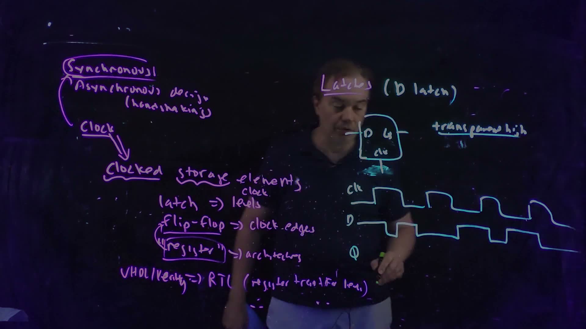
The answer the whole industry uses is synchronous design (24:23) board. Put a storage element at the boundary of every step. One global signal, the clock, tells all of them at the same moment to take in the answer of the logic before them and hold it for the logic after them. The logic between two clock ticks then always starts from steady inputs, and it has until the next tick to finish.

Two ways to sequence logic added (the board, Lecture12 @ 28:52, has the words only). (a) Synchronous: logic (the ovals) sits between flip-flops, and one clock tells every flip-flop when to capture, so each stage has exactly one cycle. (b) Asynchronous: no clock; each stage tells the next that its data is ready (req) and waits for the next to confirm it has taken it (ack): a handshake.

The board (Lecture12 @ 28:52)

Lecture12 @ 28:52Synchronous and asynchronous design; clocked storage elements: latch ⇒ levels, flip-flop ⇒ clock edges, register ⇒ architecture; VHDL/Verilog ⇒ RTL.

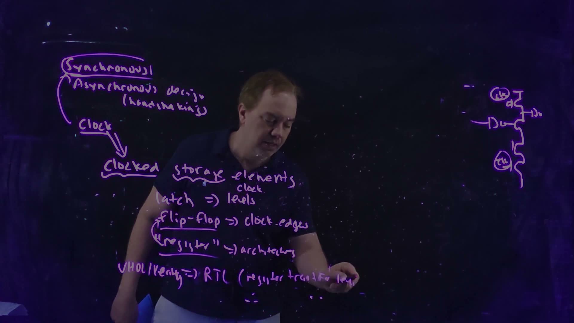
Fair copy of the board above (Lecture12 @ 28:52), mark for mark in its own layout. The board is written in one pen, so the copy is all black. The end of “(register transfer level)” is under the lecturer’s hand at 28:52; it is read from 29:48. The circuit at the right is what is left of the dynamic-logic board, a domino stage with clk on the precharge PFET and on the foot, which was erased only in part; it is copied as it stands.

The price is the clock itself. Every storage element on the chip must see its tick at the same time, so “you put a lot of burden on the clock and its distribution” (25:09). Chapter 14 measures that burden as clock skew.

Or local handshakes

The alternative is asynchronous design (25:33) board. There is no global clock. Each stage tells the next “I’m sending you data”, and the next answers “yes, I got it” (25:41): a handshake on local control signals. Data moves as soon as it is ready and the next stage can take it.

Panel (b): stages handing data on with req and ack, no clock. Original figure ↑

This term’s class gave the trade-off a name added (Fall 2026 Lecture 11, 37:31). In a synchronous design a stage that finishes early waits for the clock: dead time, in which it does nothing useful. Asynchronous design has no dead time, “but the overhead of the controls and managing all of this generally is not a win”. The class also placed asynchronous design where it does appear: large blocks or cores may be asynchronous with respect to each other, each synchronous inside. A signal that crosses between them arrives with no fixed timing to the local clock, which is the setting for metastability in Section 5.

Dead time against handshake overhead (added numbers on the class's point)

1. Two pipeline stages. Stage A takes 300 ps and stage B 480 ps, each including its storage element’s own overhead.
2. Synchronous. One clock serves both, so its period is set by the slower stage: 480 ps. Stage A finishes after 300 ps and waits $480 - 300 = 180$ ps every cycle: that is its dead time.
3. Asynchronous. Add a 100 ps handshake to each stage: A takes 400 ps and B 580 ps. A no longer waits for a clock, but B is now the bottleneck at 580 ps, so one item leaves every 580 ps.
4. The verdict. The synchronous pipeline delivers an item every 480 ps, the asynchronous one every 580 ps: 100 ps worse. Removing A’s dead time saved nothing, because the throughput is set by the slowest stage, and that stage paid the handshake. This is the class’s “generally is not a win”.

Latches, flip-flops and registers

The storage elements a clock commands are clocked storage elements (26:33) board, and there are two kinds:

• a latch responds to the clock’s levels: while the clock is at one level it passes its input through, and while it is at the other it holds (27:26);
• a flip-flop responds to the clock’s edges: it takes its input at one kind of edge and holds it until the next (27:45).

Their symbols differ only at the clock input: a plain clock input for a latch, a small triangle (a caret) for a flip-flop, and a bubble on either for the opposite polarity. Sections 2, 9 and 10 use all four.

The four clocked storage symbols (from the boards, Lecture12 @ 31:48, 36:53, 50:53 and 56:32). (a) A latch, transparent while clk = 1. (b) A bubble on the clock: transparent while clk = 0. (c) A caret marks an edge-triggered flip-flop, which samples D at the rising edge. (d) Caret and bubble: it samples at the falling edge.

A register is an architectural idea, a place that holds a value in the machine’s description (28:00). In a flop-based design every register becomes one flip-flop (one per bit), and hardware description languages such as VHDL and Verilog describe a design at the register-transfer level (RTL), explicit in its state (28:24) board. The words drift in use: many people say “latch” for a flip-flop (50:42), so read an exam’s figure, not its words.

Traps.

• “Asynchronous means no timing rules.” The handshake is a timing rule of its own, and it costs time on every transfer, which is why it usually loses.
• “Register” and “flip-flop” are the same thing. Only in a flop-based design; a register is the architectural value, the flip-flop one way to build it.
• Calling a flip-flop a latch. The lecture’s own warning (50:42). A latch is transparent for half a cycle; a flip-flop never is. Sections 2 and 9 show how different their outputs are on the same inputs.

Check yourself Two pipeline stages take 250 ps and 450 ps (overheads included). An asynchronous version adds a 120 ps handshake to each stage. Which style delivers items faster, and by how much per item?

Synchronous: the clock period is the slower stage, 450 ps. Asynchronous: the stages take 370 ps and 570 ps, and the slower one sets the rate, 570 ps per item. The synchronous pipeline is faster by $570 - 450 = 120$ ps per item: the whole handshake of the slowest stage.

Check yourself Which element's output can change while the clock stays high: a latch or a flip-flop?

A latch that is transparent while the clock is high: its output follows D for the whole high phase. A flip-flop’s output changes only just after its active edge.

2. The D latch: transparent and opaque

You need

Clock levels and edges. A clock is a square wave. While it is high (clk = 1) or low (clk = 0) it sits at a level; it changes at a rising edge (0 to 1) and a falling edge (1 to 0). Chapter 11’s dynamic gates already act on levels: they precharge while clk = 0 and evaluate while clk = 1. A latch acts on levels too, and this section reads its output from the levels of its clock.

The latch symbol. A box with the data input D, the output Q and the clock input clk at the bottom: no caret, so it is level-sensitive (Section 1).

The storage symbols (Section 1): this section uses (a), the transparent-high latch, and (b), its transparent-low twin. Original figure ↑

The question. A latch has two inputs, the data D and the clock clk. Given both waveforms, what does Q do, and how long after each cause does each change of Q appear?

Two rules

The lecture’s D latch is transparent high (29:06–30:46) board:

• clk = 1: transparent. Q follows D. Every change of D appears at Q a little later, as if the latch were a wire with a delay.
• clk = 0: opaque. Q holds. It keeps the value D had at the moment the clock fell, whatever D does afterwards.

The falling edge is therefore the moment the latch closes, and the rising edge the moment it opens.

A transparent-high D latch (redrawn from the board, Lecture12 @ 31:03 and 36:53). While clk = 1 the latch is transparent and Q follows D a short delay later; while clk = 0 it holds the value D had when clk fell, and D’s edges in that phase never reach Q. Each change of Q comes either at a rising clock edge (a clock-to-Q delay) or with a D edge inside a high phase (a D-to-Q delay).

The board (Lecture12 @ 36:53)

Lecture12 @ 36:53The D latch's waveform with Q traced, the two delays and setup and hold; the bubble on clk makes it transparent low.

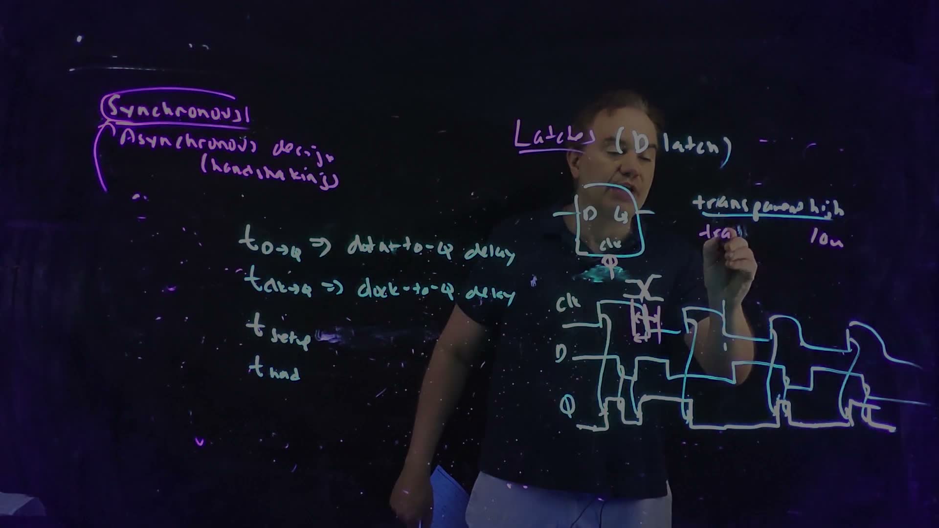
Fair copy of the board above (Lecture12 @ 36:53), mark for mark in its own layout, with the three waveform rows levelled. Black is the cyan pen of the latch board, and the purple pen of the earlier board at the top left and in “Latches”. Magenta is the pink pen, the last layer: the bubble on clk, “transparent low” and the setup and hold marks at the first falling edge. “transparent low” is still being written at 36:53 (only “tra” and “low” are on the board); it is copied as it stands, and is complete at 39:40. The thin lines join each clk or D edge to the Q edge it causes.

Reading Q edge by edge

The board’s waveform has four clock pulses, and D changes both while the clock is high and while it is low. The lecturer reads Q from left to right, starting from Q = 0 (30:46–32:16) board.

Tracing the board's latch (board, 30:46–32:16)

1. Before pulse 1 the clock is low, so the latch is opaque and Q stays at its starting 0, although D is 1.
2. Pulse 1 rises. The latch opens and D is already 1, so Q rises a little after the clock edge.
3. Inside pulse 1 D falls and rises again. The latch is transparent, so Q falls and rises with it.
4. Pulse 1 falls. The latch closes with D = 1 and holds Q = 1. While the clock is low, D falls; Q does not see it.
5. Pulse 2 rises. The latch opens on D = 0, so Q falls a little after the clock edge. D does not change during pulse 2; the latch closes holding 0, and D’s rise in the low phase after pulse 2 is ignored: “I’m not gonna see this edge at all” (31:55).
6. Pulses 3 and 4 repeat the pattern: Q rises at each rising edge (D is 1 then), and falls with D inside the pulse. D’s rise after pulse 3 is ignored.

Three D edges, all while the clock is low, never reach Q. Every other change of Q has a cause: either the clock opened the latch on a D that differed from Q, or D changed while the latch was open.

Two delays

Those two causes have two different delays (33:06–34:01) board:

• $t_{D\to Q}$tD→Q​, data-to-Q delay: the latch is already open and D changes; the change runs straight through the latch to Q.
• $t_{clk\to Q}$tclk→Q​, clock-to-Q delay: D already differs from Q while the latch is opaque; the clock opens the latch, and Q changes $t_{clk\to Q}$ after that clock edge.

Neither delay is zero, and they need not be equal: they are different paths through the circuit (Section 6 shows the transistors).

The D latch, transparent highboard

Transparent (clk = 1), a D edge at $t_D$tD​:

$$Q(t_D + t_{D\to Q}) = D(t_D)$$

Transparent, at an opening edge $t_o$ where $D \ne Q$Q:

$$Q(t_o + t_{clk\to Q}) = D(t_o)$$

Opaque (clk = 0), after a closing edge $t_c$tc​:

$$Q = D(t_c)$$

Holds when: D obeys the setup–hold window at each closing edge (Section 3); edges counted from the causing input's edge

Memorize or derive. Memorize the two rules and which delay goes with which cause. There is nothing to derive: the exam asks you to read Q off a waveform, and that is these two rules applied edge by edge.

A worked example with times

The board’s waveform has no numbers. To read the two delays off a figure, give it some added. This shared stimulus is used again in Sections 3, 9 and 10, so that a latch, a flip-flop and a master–slave pair can be compared on identical inputs:

• clk high on [2, 7), [12, 17), [22, 27) and [32, 37) ns: a 10 ns period, 50% duty;
• D = 1 at time 0, with edges at 3.5 ns ↓, 5 ns ↑, 9 ns ↓, 19 ns ↑, 24 ns ↓, 29 ns ↑ and 34 ns ↓;
• Q = 0 at time 0; $t_{clk\to Q} = 0.3$ ns, $t_{D\to Q} = 0.2$ ns (for example; real latches are tens of ps).

The board’s latch with times added, computed from the shared stimulus with $t_{clk\to Q} = 0.3$ ns and $t_{D\to Q} = 0.2$ ns. Q’s eight edges are numbered in time order. ①, ④, ⑤ and ⑦ are clock-caused: the latch opens at a rising edge and Q moves to D after $t_{clk\to Q}$tclk→Q​. ②, ③, ⑥ and ⑧ are data-caused: D changes while the latch is open and Q follows after $t_{D\to Q}$tD→Q​. The D edges marked × (9, 19 and 29 ns) arrive while clk = 0 and are ignored.

Every Q edge of the transparent-high latch (added numbers)

1. 2 ns, the clock rises. The latch opens on D = 1 while Q = 0: a clock-caused edge. Q rises at $2 + 0.3 = 2.3$ ns. ①
2. 3.5 ns, D falls inside the pulse: a data-caused edge. Q falls at $3.5 + 0.2 = 3.7$ ns. ②
3. 5 ns, D rises: Q rises at 5.2 ns. ③
4. 7 ns, the clock falls. The latch closes holding 1. D’s fall at 9 ns comes while the latch is opaque and is ignored.
5. 12 ns, the clock rises on D = 0 while Q = 1: Q falls at 12.3 ns. ④ D’s rise at 19 ns comes after the latch closed at 17 ns and is ignored.
6. 22 ns, the clock rises on D = 1: Q rises at 22.3 ns. ⑤ D falls at 24 ns inside the pulse: Q falls at 24.2 ns. ⑥ D’s rise at 29 ns is ignored.
7. 32 ns, the clock rises on D = 1: Q rises at 32.3 ns. ⑦ D falls at 34 ns: Q falls at 34.2 ns. ⑧

Q has eight edges: four clock-caused (①, ④, ⑤, ⑦ at 2.3, 12.3, 22.3 and 32.3 ns) and four data-caused (②, ③, ⑥, ⑧ at 3.7, 5.2, 24.2 and 34.2 ns), exactly as on the board. The three D edges at 9, 19 and 29 ns are ignored.

Check. Every clock-caused edge sits exactly $t_{clk\to Q} = 0.3$ ns after a rising edge (2, 12, 22, 32 ns), and every data-caused edge exactly $t_{D\to Q} = 0.2$ ns after a D edge inside a high phase. No Q edge falls in a low phase: an opaque latch cannot change its output.

Transparent low

A bubble on the clock input inverts the clock (36:44) board: the latch is transparent while clk = 0 and opaque while clk = 1. It opens at the falling edge and closes at the rising edge. The rules are the same with the levels swapped.

The storage symbols (Section 1): (a) transparent high, (b) transparent low, with the bubble on clk. Original figure ↑

Traps.

• “Q changes at the falling edge.” The falling edge is when a transparent-high latch stops following D. Q changes at a falling edge only through some earlier cause still in flight.
• One delay for every edge. Ask what caused the edge: the clock opening the latch ($t_{clk\to Q}$tclk→Q​), or D moving while it was open ($t_{D\to Q}$tD→Q​).
• $t_{clk\to Q}$ at every rising edge. Only when D already differs from Q at the opening edge; otherwise the opening changes nothing, and Q has no edge at all.
• Forgetting the starting value. Q before the first opening is whatever the latch held; the board, and this example, assume Q = 0.

Check yourself The same stimulus goes into a transparent-low latch that holds Q = 1 at time 0. Which D edges reach Q, and at what times does Q change?

A transparent-low latch is open while clk = 0: on [0, 2), [7, 12), [17, 22), [27, 32) and [37, 40) ns. At 0 ns D = Q = 1, so nothing happens. At 7 ns it opens on D = 1 = Q: no change. D falls at 9 ns while it is open: Q falls at 9.2 ns. It opens at 17 ns on D = 0 = Q; D rises at 19 ns: Q rises at 19.2 ns. It opens at 27 ns on D = 0 (D fell at 24) while Q = 1: a clock-caused edge, Q falls at 27.3 ns; D rises at 29 ns: Q rises at 29.2 ns. It opens at 37 ns on D = 0 (D fell at 34): Q falls at 37.3 ns. The D edges that reach Q (9, 19, 29 ns) are exactly the three the transparent-high latch ignored.

Check yourself In the shared stimulus, move D's fall from 24 ns to 26 ns. What does the transparent-high latch's Q do?

26 ns is still inside the pulse [22, 27), so the latch is transparent: Q falls at $26 + 0.2 = 26.2$ ns instead of 24.2 ns. Moved later than $27 - 0.4 = 26.6$ ns, it would fall inside the setup window of the closing edge at 27 ns (for $t_{setup} = 0.4$ ns), the subject of Section 3.

3. Setup, hold and the aperture

You need

The latch’s two rules (Section 2). A transparent-high latch follows D while clk = 1 and holds while clk = 0. What it holds is the value D had at the closing edge $t_c$tc​, the falling edge of the clock. A transparent-low latch (a bubble on its clock input) closes on the rising edge instead.

The transparent-high latch (Lecture12 @ 36:53, redrawn): Q follows D while clk = 1 and holds while clk = 0. Original figure ↑

The question. Section 2 said a latch keeps “the value D had at the closing edge”. What if D changes exactly at that edge? And how far from the edge must D stay for the stored value to be certain?

What gets stored

The latch stores D at its closing edge $t_c$ (34:01) board. Inside the circuit (Section 6) the closing edge turns off the switch that connects D to the storage node, and the storage loop takes over whatever voltage that node has at that moment. If D is moving then, the node is caught part-way. The result is unknown: it may be the old value, the new one, or neither for a while: “It could wind up somewhere in mid-rail and sit there for a while” (34:52). That third outcome is metastability, Section 5’s subject.

D changing inside the window: the output can hang near $V_{DD}/2$ before it resolves either way (sketch, Section 5). Original figure ↑

Keep D still around the edge

So the latch needs D steady for a short time on both sides of the closing edge (35:21–36:35) board:

• the setup time $t_{setup}$tsetup​: D must be steady for at least this long before the closing edge;
• the hold time $t_{hold}$thold​: D must stay steady for at least this long after it.

The window from $t_c - t_{setup}$ to $t_c + t_{hold}$ is the aperture, of width $t_{setup} + t_{hold}$ (36:19, 53:09). D may do anything outside it; inside it, D must not change.

The aperture of a transparent-high latch (redrawn from the board, Lecture12 @ 36:53). D must be steady from $t_{setup}$ before the closing edge $t_c$ until $t_{hold}$ after it (shaded). A change well before the window (top row, ✓) is captured cleanly; a change inside it (bottom row, ✗, the board’s X at the edge) may not be, and can leave the latch metastable.

The board (Lecture12 @ 36:53)

Lecture12 @ 36:53Setup and hold around the first falling (closing) edge of the transparent-high latch.

Fair copy of the board above (Lecture12 @ 36:53). The setup and hold marks are the three magenta bars and small arrows just right of the X, at the first falling edge. Original figure ↑

The setup–hold windowboard

$$\text{D steady on}\ \left[\,t_c - t_{setup},\ t_c + t_{hold}\,\right]$$$$\text{aperture} = t_{setup} + t_{hold}$$

Holds when: about the closing edge t_c (the falling edge for transparent high, the rising edge for transparent low); setup and hold both positive, as the lecture draws them

Memorize or derive. Memorize the window and, above all, which edge it sits on: the edge that closes the latch. For a transparent-low latch that is the rising edge (36:44).

A worked example

added A transparent-high latch closes at $t_c = 17$ ns, with $t_{setup} = 0.4$ ns and $t_{hold} = 0.2$ ns.

Testing D edges against one closing edge (added)

1. The window. From $17 - 0.4 = 16.6$ ns to $17 + 0.2 = 17.2$ ns; the aperture is $0.4 + 0.2 = 0.6$ ns.
2. D changes at 16.3 ns: before 16.6 ns, so it has settled by the setup time. Safe; the latch stores the new value.
3. D changes at 16.8 ns: inside the window, before the edge. A setup violation: D arrived too late.
4. D changes at 17.1 ns: inside the window, after the edge. A hold violation: D left too early.
5. D changes at 17.4 ns: after 17.2 ns. Safe: the latch is already opaque and ignores it until it reopens at 22 ns.

The shared stimulus (Section 2: clk high on [2, 7), [12, 17), [22, 27), [32, 37) ns; D edges at 3.5, 5, 9, 19, 24, 29 and 34 ns). The transparent-high latch closes at 7, 17, 27 and 37 ns. No D edge comes within 2 ns of any of them (the closest are 5 and 9 ns around 7 ns, 19 ns after 17 ns, and 29 ns after 27 ns): all far outside the 0.6 ns windows, so every value the latch stored in Section 2 is certain.

The shared stimulus through the transparent-high latch (computed, Section 2): closing edges at 7, 17, 27 and 37 ns, D edges well clear of them. Original figure ↑

Traps.

• The window on the opening edge. Setup and hold protect the moment the latch stops listening, the closing edge. An opening edge needs nothing: D simply flows through.
• “A violation stores the wrong value.” It may store either value, or hang near mid-rail first (Section 5). That uncertainty is the problem.
• “A slower clock fixes a hold violation.” A slower clock moves the next edge further away, which helps D arrive in time before it (setup). Hold is about D leaving too soon after the same edge, and the clock period does not appear in it (Section 11’s preview; Chapter 14).

Check yourself A transparent-low latch has t_setup = 0.3 ns and t_hold = 0.1 ns and closes at 22 ns. Which D edges violate its window: 21.6, 21.8 or 22.05 ns?

A transparent-low latch closes on the rising edge, here at 22 ns, so the window is $[22 - 0.3,\ 22 + 0.1] = [21.7, 22.1]$ ns. 21.6 ns is before it: safe. 21.8 ns is inside, before the edge: a setup violation. 22.05 ns is inside, after the edge: a hold violation.

Check yourself Why can't an input that comes from another clock domain promise to respect the window?

The window is fixed to this latch’s clock edges, and the other domain’s data changes at times set by its own clock, with no fixed relation to ours. Sooner or later one of its edges lands inside our aperture. Such inputs need a synchronizer, and Section 5 shows what can happen to it.

4. Storing a bit: static and dynamic

You need

The inverter’s transfer curve (Chapter 6). An inverter’s output is high for a low input and low for a high one, and it switches around its threshold $V_M$VM​, where output equals input (about $V_{DD}/2$ for a balanced inverter). Two inverters in a row give back the original level, cleaned up: the restoring property.

Each curve of the butterfly diagram (Section 5) is one inverter’s transfer curve: flat near the rails, steep around $V_M$ in the middle. Original figure ↑

Off transistors still leak. A transistor that is off still passes a small current, the subthreshold current of Chapter 4 (and gate leakage). Chapter 11 §8 met it as the droop of a dynamic node that nothing holds. Here it limits how long a node can store a bit on its own.

Charge on a capacitor added. A capacitance $C$ at voltage $V$ holds charge $Q = CV$CV, and a current $I$ drawn from it changes its voltage at the rate $dV/dt = I/C$I/C.

The question. Section 2’s latch “holds” its value while the clock is low. Something inside must remember it. What can remember a bit, and for how long?

The lecture names two ways (37:05–38:10) board: “Memory ① Static ② Dynamic”.

Static: a loop of two inverters

Connect two inverters in a ring: the first from node $V_1$ to node $V_2$V2​, the second from $V_2$ back to $V_1$ (38:37) board. Suppose $V_1 = 1$1. The first inverter makes $V_2 = 0$0, and the second turns that 0 back into $V_1 = 1$1: the loop agrees with itself and stays. The opposite state, $V_1 = 0$ and $V_2 = 1$1, agrees with itself too. So the loop has two states, $(V_1, V_2) = (1, 0)$ and $(0, 1)$(0,1), as the board writes beside the two nodes: it is bistable.

Each inverter actively drives its output from the supply, so a small disturbance is pulled back to the rail. The state lasts as long as the power is on, with no clock and no refresh. That is static storage, and it is the cell of an SRAM (static random-access memory, 38:10).

Two ways to store a bit (redrawn from the boards, Lecture12 @ 39:40 and 44:46). (a) Static: two inverters in a loop hold either $(V_1, V_2) = (1, 0)$ or $(0, 1)$ for as long as the supply is on, because each restores the other’s output. (b) Dynamic: with the switch off (clk = 0) the bit is only charge on $C_X$CX​, which the leakage $I_{leak}$ drains (the leakage arrow is added), so it lasts a limited time.

The board (Lecture12 @ 39:40)

Lecture12 @ 39:40Memory: ① static, the cross-coupled inverters with their two states (1, 0) and (0, 1); ② dynamic; the butterfly diagram being drawn.

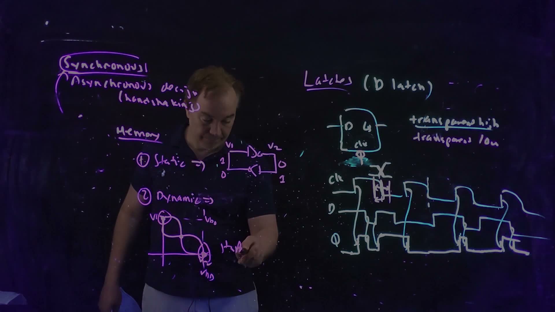
Fair copy of the board above (Lecture12 @ 39:40), mark for mark in its own layout. Black is the purple pen (the memory board in the middle, the earlier notes at the top left and “Latches”) and the cyan pen of the latch board at the right. Magenta is the latch board’s pink pen, as in the 36:53 copy: the bubble on clk, “transparent low” and the setup and hold marks. The parameter list of 36:53 has been erased to make room for the memory board. “sta” at the lower middle is the start of “stable operating point”, being written at 39:40; it is complete on the next board.

Dynamic: charge on a node

The other way is to put charge on a node and then cut the node off: a switch connects the node to the data, then opens (41:23–41:48) board. With nothing driving it, the node keeps its voltage on its own capacitance $C_X$CX​, the gate capacitance of whatever it drives plus its wiring and junctions. That is dynamic storage. It uses fewer devices, but nothing restores the level: the off switch and the gates around the node leak, and the stored charge drains away. A dynamic memory must therefore rewrite every cell before it fades, which is the refresh of a DRAM (dynamic RAM) and its refresh controller (42:16).

How long does a dynamic node last?

added The lecture gives no number; one line of circuit theory does. If a constant current $I_{leak}$ drains the node, its voltage falls at a constant rate:

Retention time (added; circuits background)

1. The node’s charge. $Q = C_X V$CX​V, so a current drawn from it changes the voltage at $dV/dt = -I_{leak}/C_X$−Ileak​/CX​.
2. A constant current gives a straight-line droop: after a time $t$t, $\Delta V = I_{leak}\,t / C_X$Ileak​t/CX​.
3. Solve for the time at which the droop reaches the most the next gate can tolerate: $t_{ret} = C_X\,\Delta V / I_{leak}$CX​ΔV/Ileak​.

Retention time of a dynamic nodeadded

$$t_{ret} \approx \frac{C_X\,\Delta V}{I_{leak}}$$

Holds when: constant leakage current (in reality it grows with temperature and with scaling); ΔV is the droop the next gate still reads correctly, for example down to its switching threshold V_M

Memorize or derive. Derive it in three lines: $I = C\,dV/dt$CdV/dt; a constant current gives a straight-line droop $\Delta V = I_{leak}t/C_X$Ileak​t/CX​; solve for $t$t.

A worked example added. A storage node of $C_X = 3$ fF leaks $I_{leak} = 0.5$ nA, and the next gate still reads a 1 correctly after a droop of 0.3 V:

$$t_{ret} = \frac{3\times10^{-15}\ \text{F} \times 0.3\ \text{V}}{0.5\times10^{-9}\ \text{A}}$$ $$t_{ret} = 1.8\ \mu\text{s}$$

A latch clocked every nanosecond rewrites its node about 1800 times within that ($1.8\ \mu\text{s}/1\ \text{ns}$1.8 μs/1 ns), so the leak never matters while the clock runs. Stop the clock for longer than about 1.8 µs, as a power-saving mode might, and the bit is lost. A static loop has no such limit.

Traps.

• “Static means unclocked.” A static latch is still clocked: the clock decides when it listens. “Static” says only how it holds the bit, by active feedback rather than by charge.
• “A faster clock means longer retention.” Retention is set by $C_X$CX​, the leakage and the tolerable droop. The clock only decides how often the node is rewritten.
• SRAM needs refresh. No: only DRAM, whose cells are dynamic (42:16).

Check yourself A dynamic node of 2 fF leaks 1 nA. It is written to V_DD = 1 V, and the next inverter's threshold is V_M = 0.5 V. How long until a stored 1 reads as a 0?

The 1 is lost when the node droops from 1 V to the threshold 0.5 V, so $\Delta V = 0.5$ V. Then $t_{ret} = C_X\,\Delta V/I_{leak} = 2\times10^{-15} \times 0.5 / 10^{-9} = 1\ \mu$s.

Check yourself At a hotter corner the leakage doubles. What happens to the retention time, and why does that matter more as transistors shrink?

$t_{ret}$ is inversely proportional to $I_{leak}$Ileak​, so it halves. Scaling raises leakage (lower thresholds, thinner oxides) and shrinks $C_X$CX​, both of which cut $t_{ret}$tret​: one reason designers stopped trusting dynamic storage in logic (Section 6).

5. Two stable points and a metastable one

You need

The static loop (Section 4). Two inverters in a ring, from $V_1$ to $V_2$ and from $V_2$ back to $V_1$V1​, hold either $(V_1, V_2) = (1, 0)$ or $(0, 1)$(0,1).

Static storage in a loop of two inverters (a) and dynamic storage as charge on $C_X$ (b) (Lecture12 @ 39:40, redrawn). Original figure ↑

The slope of the transfer curve (Chapter 6). An inverter’s curve is flat near the rails, where its slope is small (magnitude below 1), and steep around its threshold $V_M$VM​, where the magnitude of its slope is well above 1. The points of slope −1 separate the two regions. A small change of the input near $V_M$ comes out amplified; near the rails it comes out shrunk.

The question. Section 4 said the loop has two states. Is that all? And what happens to a latch whose data changes right at its closing edge (Section 3), so that the loop is left somewhere in between?

The butterfly diagram

Draw both inverters of the loop on one pair of axes (38:37–41:04) board.

Building the butterfly (board, 38:37–41:04)

1. Inverter A takes $V_1$ and drives $V_2$V2​: $V_2 = f(V_1)$f(V1​), its transfer curve.
2. Inverter B takes $V_2$ and drives $V_1$V1​: $V_1 = f(V_2)$f(V2​). On the same axes it is inverter A’s curve mirrored across the diagonal $V_1 = V_2$V2​, because the roles of the two axes are swapped.
3. A state of the loop must satisfy both inverters at once, so it lies on both curves: it is an intersection.
4. The two curves cross three times board: at the top left ($V_1 = V_{DD}$V1​=VDD​, $V_2 = 0$0, the stored 1), at the bottom right ($V_1 = 0$V1​=0, $V_2 = V_{DD}$VDD​, the stored 0), and once in the middle, where both nodes sit near $V_M$VM​.

The picture looks like a pair of wings, hence its name, the butterfly diagram (41:04). The board labels the outer crossings “stable operating point” and the middle one “metastable state”.

The butterfly diagram of two cross-coupled inverters (redrawn from the board, Lecture12 @ 41:40): one inverter’s curve and the other’s, mirrored across the dotted diagonal $V_1 = V_2$V2​. They cross three times. The outer points, $(V_1, V_2) = (1, 0)$ and $(0, 1)$(0,1), are the stable states that store a bit; the middle one (hollow), at $V_{DD}/2$ on the diagonal, is metastable. The curves are computed from an illustrative $f(v) = V_{DD}/(1 + e^{12(v/V_{DD} - 1/2)})$e12(v/VDD​−1/2)), not a device model; the board’s horizontal axis is unnamed, and $V_2$ is this guide’s name for it.

The board (Lecture12 @ 41:40)

Lecture12 @ 41:40The butterfly diagram: two stable operating points and a metastable state in the middle.

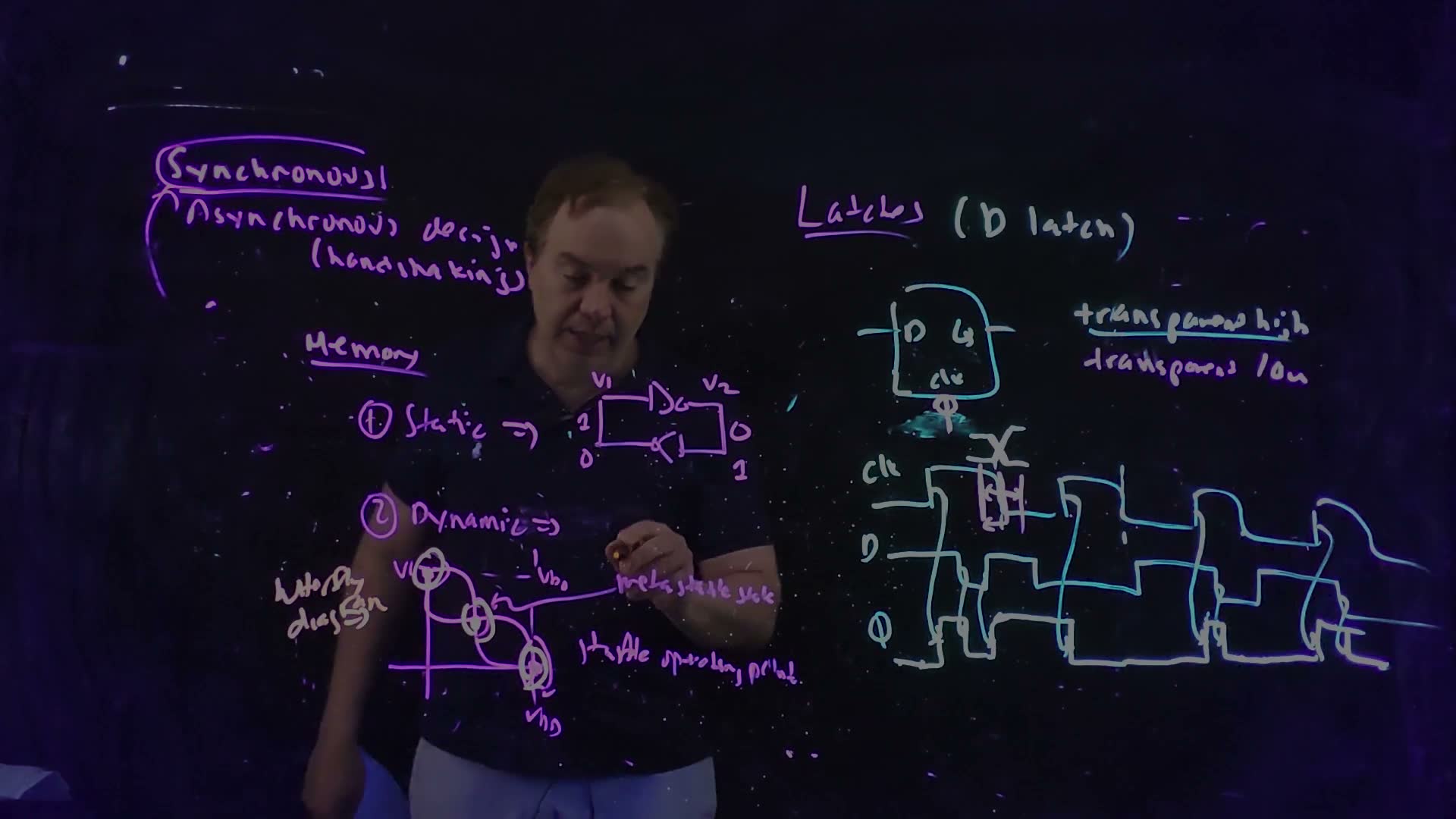
Fair copy of the board above (Lecture12 @ 41:40), mark for mark in its own layout. Black is the purple pen (the memory board, the earlier notes and “Latches”), the cyan pen of the latch board, and the orange pen of “butterfly diagram” at the left. Magenta is the latch board’s pink pen, as in the 36:53 and 39:40 copies: the bubble on clk, “transparent low” and the setup and hold marks. Since 39:40 the middle crossing has been circled, every crossing circled a second time, and the two labels added.

States of the cross-coupled pairboard

$$V_2 = f(V_1) \quad\text{and}\quad V_1 = f(V_2)$$

Holds when: DC picture: each node settled; f is the inverter's transfer curve (the same for both inverters here)

Why the middle point does not hold

“In this sort of DC static picture, I can’t prove this to you, but this particular state is not stable” (40:03). The DC curves only say where the loop can sit still. Whether it stays depends on what a small disturbance does, and a short argument from the slopes shows it added.

Follow a small nudge around the loop (added)

1. Nudge $V_1$ by a small $\delta$ away from a crossing point.
2. Inverter A passes the change to $V_2$ multiplied by its slope there, $A_A$ (negative: an inverter).
3. Inverter B passes it back to $V_1$ multiplied by its slope, $A_B$AB​. After one trip around the loop the nudge is $A_A A_B\,\delta$AA​AB​δ. Both slopes are negative, so the product is positive: the nudge keeps its sign.
4. At an outer point both inverters sit on the flat part of their curves, so $|A_A A_B| < 1$1: each trip shrinks the nudge and it dies out. The point is stable.
5. At the middle point both sit on the steep part, so $A_A A_B > 1$1: each trip grows the nudge, and the loop runs away from the middle until it reaches one of the outer points. The point is metastable: it can balance there, but the slightest noise tips it.
6. How long it takes depends on how small the first nudge was. The smaller the nudge, the more trips it needs to grow to a full level: “How long that’s going to take to happen is … somewhat indeterminate” (40:20).

Loop gain at a crossing (an illustration, not a timing model)added

$$\delta \;\to\; A_A\,\delta \;\to\; A_A A_B\,\delta$$$$\text{unstable when } A_A A_B > 1$$

Holds when: small disturbances only; the two slopes are taken at the crossing; the board states only that the middle point is not stable

Memorize or derive. Memorize the picture: two curves, three crossings, the outer two stable, the middle one metastable. Derive the reason if a question asks why: follow a nudge $\delta$ once around the loop; it comes back as $A_AA_B\,\delta$AA​AB​δ, and at the middle point $A_AA_B > 1$1.

An illustration with numbers added. This is not a timing model: the course gives no time constant for resolving metastability, and none is used here. Take, for example, inverters whose slope at $V_M$ is −4, so that the loop gain at the middle point is $(-4)(-4) = 16$16, with $V_{DD} = 1.2$ V.

How many trips to fall out of the middle (added illustration)

1. A 10 mV nudge becomes $16 \times 10 = 160$ mV after one trip around the loop.
2. A full fall needs the nudge to reach about $V_{DD}/2 = 0.6$ V away from the middle. After $n$ trips the nudge is $16^n\,\delta$16nδ, so $n = \ln(0.6\ \text{V}/\delta)/\ln 16$ln(0.6 V/δ)/ln16: about 1.5 trips for 10 mV.
3. Smaller nudges need more: 1 mV needs about 2.3 trips, 1 µV about 4.8.
4. The moral. The closer D’s change is to the closing edge, the more evenly the loop is left balanced, the smaller the nudge and the longer the hang. There is no upper limit: an edge timed exactly enough could keep the loop near the middle for as long as you like. That is why the time is “indeterminate”.

Where a latch meets it

A latch meets the middle point when D changes inside its aperture (Section 3): the closing edge leaves node X part-way, and the loop starts near the middle. The output can then sit near mid-rail for a while before it falls to a 1 or a 0, and nobody can say which or when.

Metastability, a sketch added. D changes inside the aperture (shaded) around the edge $t_c$ at which the element decides what to keep, so the storage loop starts near its balance point: Q rises only to about $V_{DD}/2$ and hangs there for an unpredictable time before it resolves to 1 or to 0 (dashed).

Inside one synchronous design this is prevented by obeying setup and hold (40:52). The hard case is an input with no fixed timing to the local clock, from another clock domain or the outside world: sooner or later one of its edges lands in the aperture. The circuit that samples such inputs is a synchronizer, and it can land in the metastable state (40:33) board. This term’s class added that synchronizers are notoriously hard to get right (Fall 2026 Lecture 11, 54:26); this course treats them qualitatively.

Traps.

• “Metastable is a third stored value.” It is a balance point the loop always leaves; only when and to which side are unknown.
• “Setup and hold remove metastability.” Only for inputs that can obey them. An asynchronous input cannot promise to.
• “The butterfly proves stability.” The lecturer’s own warning (40:03): the DC curves show where the loop can rest, not whether it stays. The slopes, through the loop gain, decide that.

Check yourself Suppose each inverter's slope never exceeded 0.5 in magnitude, even at its threshold. How many times would the two curves cross, and could the loop store a bit?

Each trip around the loop would multiply a nudge by at most $0.5 \times 0.5 = 0.25$0.25, so every disturbance would die out and the loop would settle to a single point. Curves that shallow cross only once, near the middle (with the drawing aid of the butterfly figure and a slope of −0.5 there is exactly one crossing). One state is no memory: the loop could not store a bit. Bistability needs a loop gain above 1 in the middle.

Check yourself With a loop gain of 16, how many more trips around the loop does a nudge 16 times smaller need to fall out of the middle?

One. Each trip multiplies the nudge by 16, so the first extra trip brings the smaller nudge up to the larger one’s size, and from there it is the same story.

6. Building the D latch from a switch and inverters

You need

A pass transistor (Chapter 10). An NFET whose gate is high connects its two terminals; with its gate low it disconnects them. It passes a 0 fully, but a 1 only up to $V_{DD} - V_T$VT​, because it turns off once its source rises to within a threshold of its gate.

Two ways to store (Section 4). Statically, in a loop of two inverters that restores its own levels; dynamically, as charge on a node’s capacitance $C_X$CX​, which leaks away.

Static storage in a loop of two inverters (a) and dynamic storage as charge on $C_X$ (b) (Lecture12 @ 39:40, redrawn). Original figure ↑

The question. How do you turn Section 4’s storage into Section 2’s latch: something that follows D while clk = 1 and holds while clk = 0?

A switch, then storage

The static and the dynamic D latch (board, 42:22–43:53)

1. A clocked switch. A pass NFET between D and an internal node X, its gate on clk (42:44) board. With clk = 1 it conducts and X follows D: transparent. With clk = 0 it is off and X is cut off from D: opaque.
2. Static: add the loop. X drives an inverter whose output is $\overline{Q}$Q​, and a second inverter feeds $\overline{Q}$ back to X (43:01) board. While the switch is off, this cross-coupled pair holds X exactly as Section 4’s loop does, at a full level, for as long as the power is on.
3. Dynamic: drop the feedback inverter. X drives one inverter to $\overline{Q}$ and nothing else (43:20) board. While the switch is off, X keeps its value as charge on its capacitance, which the board marks “capacitor”.
4. Polarity. Both latches deliver $\overline{Q}$Q​, the complement of the stored bit. An extra inverter gives Q when the true polarity is needed (43:01).

The two D latches (redrawn from the board, Lecture12 @ 44:46). (a) Static: while clk = 1 the pass NFET writes D onto X; while clk = 0 the feedback inverter holds X. (b) Dynamic: while the pass NFET is off the value is only charge on the node capacitance $C_X$ (the board’s “capacitor”), so it leaks away. Both deliver $\overline{Q}$Q​.

The board (Lecture12 @ 44:46)

Lecture12 @ 44:46The static D latch (top: pass NFET into cross-coupled inverters) and the dynamic D latch (bottom: the state on the node's capacitance).

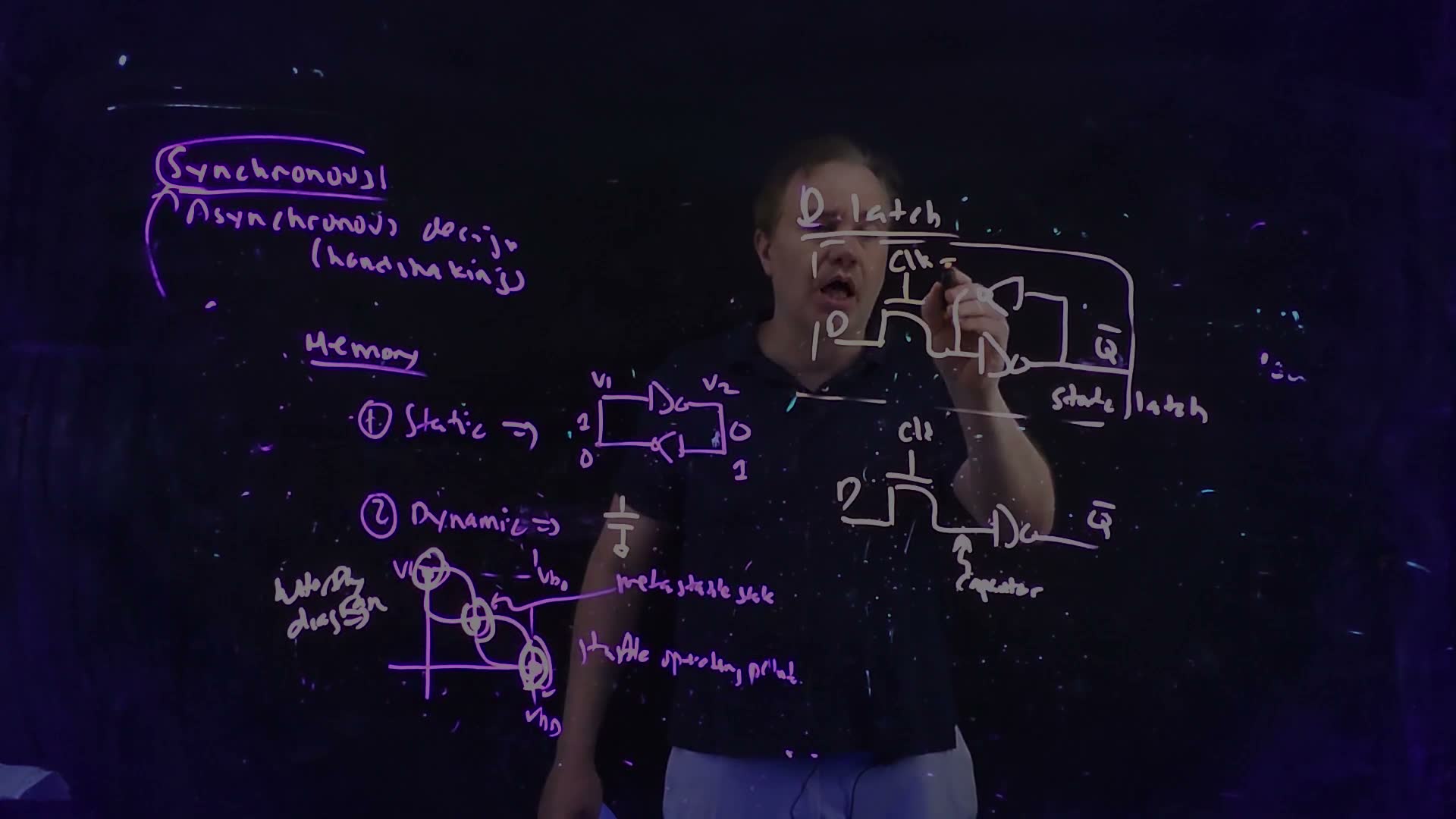
Fair copy of the board above (Lecture12 @ 44:46), mark for mark in its own layout. The board has two pens, both copied in black: the purple pen of the memory board and the earlier notes, and the pale orange pen (the one of “butterfly diagram”) of the D latch board at the right and the capacitor drawn after “② Dynamic ⇒”. The latch board of 36:53 has been erased. The lone bar after “clk” over the static latch is “clk = 1” being written; it is complete by 46:09. The box round the static latch is drawn faintly, with gaps, and is copied as it stands.

The transistor counts follow: the static latch is one pass NFET and two inverters, 1 + 4 = 5 transistors (7 with a Q inverter); the dynamic latch is one pass NFET and one inverter, 1 + 2 = 3 (5 with a Q inverter).

Why designers avoid the dynamic latch

The dynamic latch is smaller and, with no loop to fight (Section 7), easy to write. Yet “these are extremely risky. I only know of one processor, the famous Alpha processor, that actually used dynamic latches” (43:29–43:53), and today’s transistors are “far too leaky” (43:59). This term’s class named the two reasons added (Fall 2026 Lecture 11, 49:49–51:23):

• leakage: the floating node forgets its value (Section 4’s retention time), and the problem gets worse with every technology generation;
• noise: a floating node is as sensitive to coupling and supply noise as a dynamic gate’s (Chapter 11 §10–§12). In a logic gate a flipped node is one wrong answer; in a storage element it is a wrong state, and the machine is dead.

So dynamic storage lives on only in DRAM, where it is refreshed by design.

A worked example added. Write a 1 into each latch with $V_{DD} = 1.0$ V, a pass NFET with $V_T = 0.3$ V and a forward inverter that switches at $V_M \approx 0.5$ V, then open the switch.

Writing a 1 through the pass NFET (added)

1. During the write (clk = 1) X rises only to $V_{DD} - V_T = 1.0 - 0.3 = 0.7$ V: the pass NFET turns off as X approaches a threshold below its gate.
2. Static latch. 0.7 V is above the forward inverter’s threshold of 0.5 V, so, provided the write wins its fight with the feedback inverter (Section 7), $\overline{Q}$ falls, the feedback inverter’s output rises, and it pulls X the rest of the way to the full 1.0 V. When clk falls, the loop holds 1.0 V.
3. Dynamic latch. Nothing restores the level. X stays at 0.7 V when the switch opens and then droops with leakage, with less margin above the next gate’s threshold than a full level would give.

Traps.

• The output is Q. Both board latches give $\overline{Q}$Q​; check the polarity before using the output.
• “A cross-coupled pair is a latch.” Not on its own: it needs the clocked switch, the only way to write it and the only part that knows about the clock.
• A full 1 through an NFET. A lone pass NFET leaves $V_{DD} - V_T$ on X. The static latch’s loop repairs it; the dynamic latch cannot.

Check yourself A dynamic latch has V_DD = 1.0 V, a pass NFET with V_T = 0.3 V, C_X = 3 fF and I_leak = 0.5 nA, and its inverter switches at V_M = 0.5 V. How long does a written 1 survive?

The written 1 is only $1.0 - 0.3 = 0.7$ V, and it is lost at 0.5 V, so the allowed droop is $\Delta V = 0.2$ V. Then $t_{ret} = C_X\,\Delta V/I_{leak} = 3\times10^{-15} \times 0.2 / 0.5\times10^{-9} = 1.2\ \mu$s, shorter than the 1.8 µs a 0.3 V droop allowed in Section 4: the degraded high costs margin.

Check yourself What does the static latch have that the dynamic one does not, and what problem does it bring?

A feedback inverter, which holds and restores X. But while clk = 1 that inverter is still on, still driving X toward the old value, so every write has to overpower it: Section 7’s write fight.

7. Writing the static latch: the fight

You need

The static D latch (Section 6). A pass NFET on clk connects D to the storage node X; X drives the forward inverter to $\overline{Q}$Q​, and a feedback inverter drives $\overline{Q}$ back onto X. The feedback inverter is always on.

The static (a) and dynamic (b) D latch (Lecture12 @ 44:46, redrawn). Original figure ↑

Device strength as resistance (Chapter 7). A turned-on NFET of width $W$ (in µm) pulling down acts like a resistance $R/W$R/W, and a PFET pulling up like $2R/W$2R/W, where $R$ is the “resistance” of a 1 µm NFET. Devices in series add their resistances.

An NFET pulling up is weak (Chapter 10; Chapter 11 §2’s resistor model). It loses overdrive as its source rises, so it pulls up like about $2R/W$2R/W, and it stops at $V_{DD} - V_T$VT​.

The switching threshold (Chapter 6). An inverter’s output flips when its input crosses $V_M$VM​, about $V_{DD}/2$ for a balanced inverter.

The same fight once before (Chapter 11 §8–§9). A half latch holds a dynamic node high, and the pull-down network must overpower it to evaluate; that is why the half latch is made weak.

The question. To write the static latch, D must drive X through the pass NFET. But the feedback inverter is still on and still driving X toward the old value. Who wins, and what if the wrong side does?

Who fights whom

The board’s scene (44:28–45:16) board: the latch holds a 1, so X = 1 and $\overline{Q} = 0$0. A driver inverter in front of it now pulls its output, the latch’s D, from 1 to 0, and clk = 1 so the pass NFET is on.

Writing a 0 into a static latch that holds 1 (redrawn from the board, Lecture12 @ 46:54). With clk = 1 the pass NFET is on, and the driver pulls D from 1 to 0 (down arrow). The feedback inverter is drawn as its two transistors: its PFET, gated by $\overline{Q} = 0$0, is on and holds X at 1 (up arrow); its NFET is off (grey). The write succeeds only if the driver and the pass NFET pull X below the forward inverter’s switching threshold against that PFET.

The board (Lecture12 @ 46:54)

Lecture12 @ 46:54The write fight: the driver pulls down through the pass NFET while the feedback inverter's PFET holds the node up; 'writeability'.

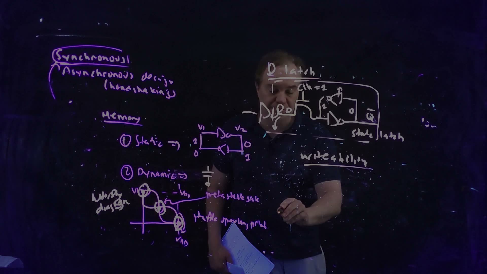
Fair copy of the board above (Lecture12 @ 46:54), mark for mark in its own layout. Both pens are copied in black: the purple pen of the memory board and the earlier notes, and the pale orange pen of the D latch board. Since 44:46 the dynamic latch has been erased, and the write fight added: the driver inverter with its “0” and down arrow, “clk = 1”, the stored state (1 on the node, 0 on Q̄), the up arrow on the feedback inverter’s back for its PFET, and “writeability”. The driver’s bubble is the small U drawn across the left side of the box.

The fight (board, 44:43–45:46)

1. Pulling X up: the feedback inverter’s PFET. Its gate is $\overline{Q} = 0$0, so it is fully on, connecting X to $V_{DD}$VDD​.
2. Pulling X down: the pass NFET (gate clk = 1) in series with the driver’s NFET (its input is now 1), connecting X to ground. “This NFET here has to overpower the PFET of this feedback path” (44:43).
3. Both are on at once, so X settles somewhere between the rails, wherever the two pulls balance.
4. If X gets below $V_M$VM​, the forward inverter flips and $\overline{Q}$ rises. That turns the feedback PFET off and its NFET on, so the feedback now pulls X down too: positive feedback finishes the write.
5. If X stalls above $V_M$VM​, $\overline{Q}$ never flips. When clk falls, the pass NFET turns off and the feedback PFET pulls X back to 1: the latch “might not be writable” (45:19) board.
6. Even a write that succeeds is costly. While both sides are on, current flows straight from $V_{DD}$ through the PFET, X, the pass NFET and the driver to ground: “the fact that I have to fight this device … will slow the latch down and will cause it to burn more power” (45:46, paraphrased).

Estimating the fight with a divider

added The lecture states the fight in words. An estimate with the course’s resistances shows how lopsided it can be. Treat each turned-on device as a resistor: then X is the middle of a resistor divider between $V_{DD}$ and ground. This is rough: real transistors are not linear resistors, so the estimate compares strengths and does not predict X’s voltage exactly.

The write fight as a divider added. (a) While a 0 is written into a latch that holds 1, three devices conduct in series: the feedback PFET pulls X up; the pass NFET and the driver’s NFET pull it down (the devices that are off are left out). (b) Each device as a resistance, an NFET of width $W$ as $R/W$ and a PFET as $2R/W$2R/W: $V_X = V_{DD}\,R_{down}/(R_{up} + R_{down})$Rdown​). The write succeeds when $V_X$ falls below the forward inverter’s switching threshold.

The divider (added)

1. The pull-up is the feedback PFET of width $W_{fb}$Wfb​: $R_{up} = 2R/W_{fb}$2R/Wfb​.
2. The pull-down is the pass NFET of width $W_{pass}$ in series with the driver NFET of width $W_{drv}$Wdrv​: $R_{down} = R/W_{pass} + R/W_{drv}$R/Wdrv​.
3. The divider. The same current flows through both, so X sits at the fraction of $V_{DD}$ that the lower resistance takes: $V_X = V_{DD}\,R_{down}/(R_{down} + R_{up})$Rup​).
4. The test. The write succeeds when $V_X < V_M$VM​. With $V_M = V_{DD}/2$ that is simply $R_{down} < R_{up}$Rup​: the pull-down path must be the stronger one.

The write fight as a resistor divideradded

$$V_X \approx V_{DD}\,\frac{R_{down}}{R_{down} + R_{up}}$$$$R_{down} = \frac{R}{W_{drv}} + \frac{R}{W_{pass}}$$$$R_{up} = \frac{2R}{W_{fb}}$$$$\text{writable if } V_X < V_M$$$$\text{with } V_M = V_{DD}/2:\quad R_{down} < R_{up}$$

Writing a 0 (the lines above): the driver’s NFET and the pass NFET pull down, the feedback PFET pulls up. Writing a 1, the roles swap, and the write succeeds if $V_X > V_M$VM​:

$$R_{up} = \frac{2R}{W_{drv}} + \frac{2R}{W_{pass}}$$$$R_{down} = \frac{R}{W_{fb}}$$

(the driver’s PFET and the pass NFET pulling up, about $2R/W$2R/W; the feedback NFET pulling down).

Holds when: widths are those of the devices that conduct; rough: every fighting device fully on and treated as a linear resistor R/W (NFET down), 2R/W (PFET up, or NFET pulling up); compares strengths, does not predict exact voltages; the writer must win before the loop's positive feedback helps

Memorize or derive. Memorize the condition in words, as the board gives it: the write path must overpower the feedback device. Derive the estimate when a question wants a number: series resistances add, then a divider, in three lines (steps 1–3).

A worked example: an unwritable latch, and two fixes

added Size everything as a “normal” designer might: all three inverters (driver, forward and feedback) 2/1 (PFET 2 µm, NFET 1 µm), and a 1 µm pass NFET. This is FN19-9’s circuit, with sizes chosen here (the exam gives none).

Write a 0, original sizes (added)

1. Pull-down. Driver NFET 1 µm and pass NFET 1 µm in series: $R_{down} = R/1 + R/1 = 2R$2R.
2. Pull-up. Feedback PFET 2 µm: $R_{up} = 2R/2 = R$R.
3. The divider. $V_X = V_{DD} \cdot 2R/(2R + R) = \tfrac23 V_{DD}$32​VDD​, above $V_M = \tfrac12 V_{DD}$21​VDD​. The forward inverter never flips: not writable. The feedback PFET, alone, is twice as strong as the two NFETs in series.

Fix A: weaken the feedback inverter. Shrink it to 0.5/0.25 µm. Now $R_{up} = 2R/0.5 = 4R$4R, and $V_X = V_{DD} \cdot 2R/(2R + 4R) = \tfrac13 V_{DD}$31​VDD​: well below $V_M$VM​, so the write succeeds. This is Chapter 11’s half-latch lesson again: the keeper must be weak.

Fix B: strengthen the write path. Widen the driver NFET and the pass NFET to 2 µm and leave the feedback alone. Now $R_{down} = R/2 + R/2 = R = R_{up}$ and $V_X = \tfrac12 V_{DD}$21​VDD​: exactly at the threshold. That is not a fix: noise or a slow corner tips it either way. Widening only the pass NFET helps even less, because the driver is in series. Wider still does work for the 0: driver and pass NFETs of 4 µm give $R_{down} = R/4 + R/4 = 0.5R$ and $V_X = \tfrac13 V_{DD}$31​VDD​. The 1 is the hard part (next): against the 1 µm feedback NFET it takes a 4 µm pass NFET and an 8 µm driver PFET, $R_{up} = 2R/8 + 2R/4 = 0.75R$0.75R, just to reach $V_X = R/(R + 0.75R) = \tfrac47 V_{DD}$74​VDD​.

The other direction: writing a 1. Now X = 0 and $\overline{Q} = 1$1, so the feedback inverter’s NFET holds X low, and the write must pull X up through the driver’s PFET and the pass NFET. A pass NFET pulls up weakly, about $2R/W$2R/W, and only to $V_{DD} - V_T$VT​.

The write-0 divider (Lecture12 @ 46:54, redrawn as resistors). For writing a 1 the roles swap: the driver’s PFET ($2R/W_{drv}$2R/Wdrv​) and the pass NFET pulling up (about $2R/W_{pass}$2R/Wpass​) form $R_{up}$Rup​, and the feedback inverter’s NFET ($R/W_{fb}$R/Wfb​) forms $R_{down}$Rdown​; the write needs $V_X$ above $V_M$VM​. Original figure ↑

Write a 1 (added)

1. Original sizes. Pull-up: driver PFET $2R/2 = R$ plus the pass NFET pulling up, $2R/1 = 2R$2R: $3R$ in all. Pull-down: feedback NFET $R/1 = R$R. $V_X = V_{DD} \cdot R/(R + 3R) = \tfrac14 V_{DD}$41​VDD​, far below $V_M$VM​: the 1 fails even worse than the 0 did.
2. With fix A the feedback NFET is 0.25 µm, $R/0.25 = 4R$4R. $V_X = V_{DD} \cdot 4R/(4R + 3R) = \tfrac47 V_{DD} = 0.571\,V_{DD}$0.571VDD​: above $V_M$VM​, so it writes, barely.
3. And the ceiling. Whatever the sizes, the pass NFET cannot lift X above $V_{DD} - V_T$ (0.7 V for $V_{DD} = 1.0$ V, $V_T = 0.3$ V). Writing a 1 through an NFET is the harder direction; check both.

Check. The estimate agrees with the lecture’s words: with equal-looking sizes the single PFET beats two NFETs in series, so a latch designed without thinking about the fight fails (45:19). And it agrees with Chapter 11’s half latch, whose keeper is sized at about a tenth of the pull-down’s strength for the same reason.

The same story in the butterfly

This term’s class drew the write on the butterfly diagram added (Fall 2026 Lecture 11, 56:55–59:14). Take $V_1$ = X, the node the writer pulls on. While the writer pulls X down, the curve of the inverter that drives X (the feedback inverter) is pulled down with it. A weak writer only dents the curve: three crossings remain, including the old state, and when the clock closes the latch falls back into it. A strong writer pulls the curve so far that the old state’s crossing disappears: only the new state is left, and the loop must go there.

A write seen on the butterfly diagram added (this term’s class, Fall 2026 Lecture 11). The writer pulls node $V_1$ (= X) down, which squashes the curve of the inverter driving it to $V_1 = a\,f(V_2)$ (thick; dashed, the undisturbed curve). With a weak writer ($a = 0.7$a=0.7, left) three crossings remain and the old state $(1, 0)$ survives, only disturbed: the write fails when the clock closes. With a strong writer ($a = 0.35$a=0.35, right) only the crossing $(0, 1)$ is left, so the loop must flip. A sketch computed from the butterfly figure’s illustrative curve, not a device model.

That is the bridge to SRAM. An SRAM cell is this ungated cross-coupled pair, accessed through pass transistors, and it lives with the write fight because density matters more than anything else in a memory (46:01–46:27). Chapter 19 sizes the cell, and also checks that reading it does not upset it (the class’s read stability).

Traps.

• Strengthening the forward inverter. It does not fight; the feedback inverter does.
• Widening only the pass NFET. The driver is in series with it, and both must be strong.
• Checking only the write-0 direction. Writing a 1 through an NFET is weaker and capped at $V_{DD} - V_T$VT​.
• “X moved, so it is written.” X must cross $V_M$ before the clock closes, or the loop restores the old value.
• “SRAM solves this with gated feedback.” SRAM does not: it keeps the bare cross-coupled pair and sizes it carefully (Chapter 19).

Check yourself In the original latch (driver and pass NFETs 1 µm), how wide may the feedback PFET be before writing a 0 becomes impossible? Use V_M = V_DD/2.

Writing a 0 needs $R_{up} > R_{down} = 2R$2R. With $R_{up} = 2R/W_{fb}$ that means $2R/W_{fb} > 2R$2R, so $W_{fb} < 1$ µm. At exactly 1 µm the write is marginal ($V_X = V_{DD}/2$VX​=VDD​/2); this example’s 2 µm is twice too wide.

Check yourself Why does the fight burn power even when the write succeeds?

While the writer and the feedback device are both on, they form a path from $V_{DD}$ through the feedback PFET, X, the pass NFET and the driver’s NFET to ground. Current flows through it until the latch flips, as in a pseudo-NMOS gate (Chapter 10) whose PFET and NFETs are both on. A stronger fight lasts longer and draws more.

8. Gated feedback: the standard-cell latch

You need

The write fight (Section 7). In the static latch the feedback inverter is always on, so writing means overpowering it: the latch can be slow, power-hungry or even unwritable.

The write fight (Lecture12 @ 46:54, redrawn): the feedback PFET holds X at 1 while the driver and the pass NFET pull it down. Original figure ↑

A transmission gate (Chapter 10, Chapter 11). An NFET and a PFET in parallel, with their gates on complementary signals (here clk and $\overline{\text{clk}}$clk). Both conduct together or neither does, and together they pass both a full 0 and a full 1.

The question. The fight exists only because the feedback is on while we write. Can we switch the feedback off exactly when we write?

Switch the feedback off while writing

Gating the feedback (board, 46:55–48:05)

1. A second switch, in the loop. Put another pass device between the feedback inverter and X, and gate it with $\overline{\text{clk}}$ (47:02) board: “I put another pass transistor here … And I gate this with clock bar”.
2. clk = 1, writing. The input switch is on and the feedback switch is off. X follows D, and nothing fights: “it kind of looks like a dynamic latch … during the write”, as this term’s class put it added (Fall 2026 Lecture 11, 59:46).
3. clk = 0, holding. The input switch is off and the feedback switch is on, so the loop closes and holds X statically.
4. Make both switches complementary (47:37) board. Since $\overline{\text{clk}}$ is already there, turn each pass NFET into a transmission gate. Full levels pass both ways, the latch is faster, and X is never pulled up through an NFET alone (47:59, paraphrased): Section 7’s weak write-1 disappears too.

The static latch with gated feedback (redrawn from the board, Lecture12 @ 48:35). The input transmission gate conducts while clk = 1 (NFET gate clk, PFET gate $\overline{\text{clk}}$clk); the feedback transmission gate conducts while clk = 0 (NFET gate $\overline{\text{clk}}$clk, PFET gate clk). Writing (clk = 1), D drives X with the feedback cut; holding (clk = 0), D is cut off and the loop through the feedback inverter holds X.

The board (Lecture12 @ 48:35)

Lecture12 @ 48:35'writeability': the gated-feedback latch (bottom), with transmission gates on clk and clk-bar.

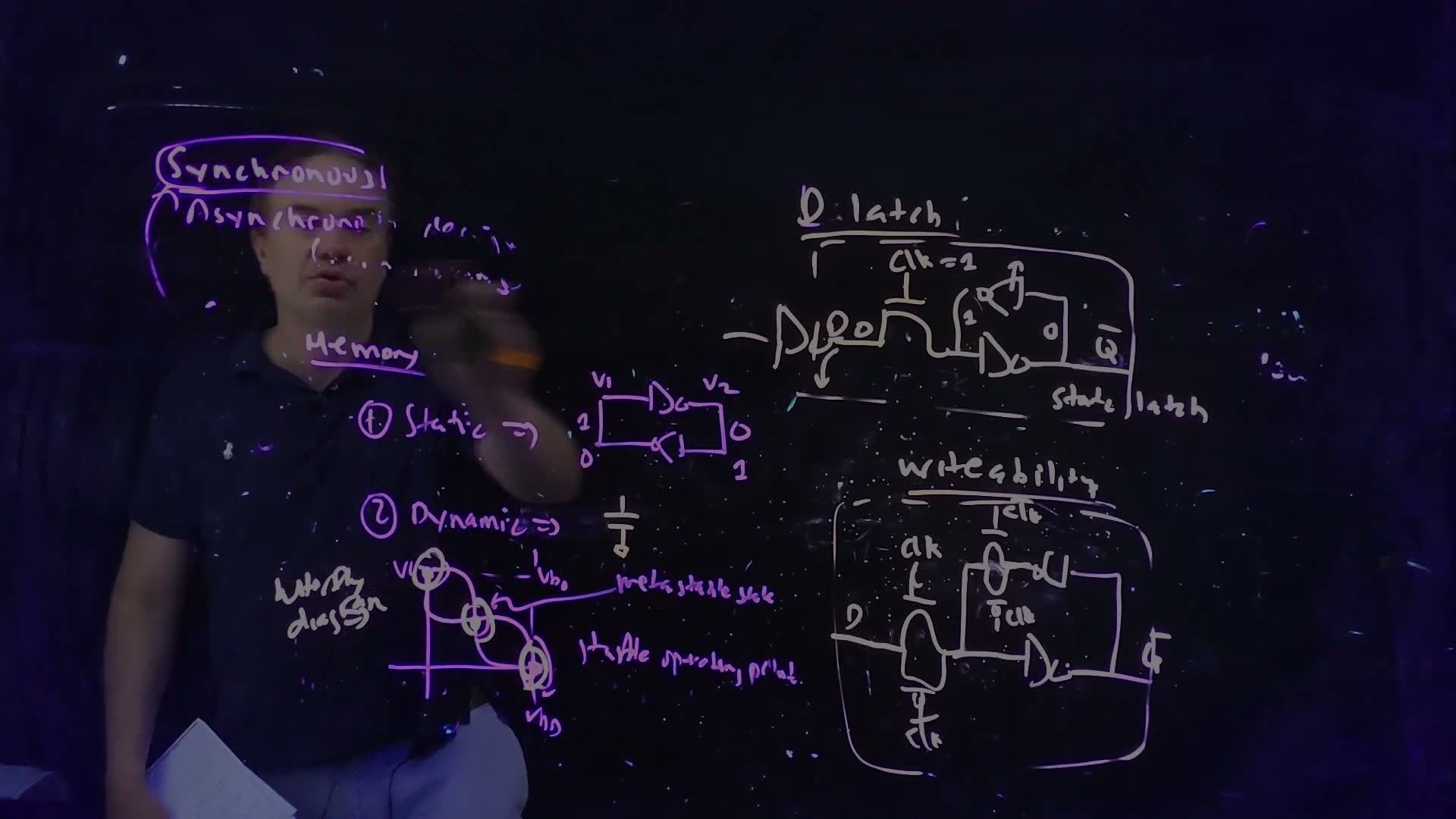
Fair copy of the board above (Lecture12 @ 48:35), mark for mark in its own layout. Both pens are copied in black: the purple pen of the memory board and the earlier notes, and the pale orange pen of the latch boards. New since 46:54 is the gated latch under “writeability”. The lecturer’s head and arm hide “Asynchronous design (handshaking)” at the top left; it is restored from 46:54. The bar over the second gate’s top “clk” runs into the box’s top line on this frame; it is read from 47:50.

The gated latch in its two phases, each transmission gate drawn as a switch added. With clk = 1 (left) the input switch is closed and the feedback switch open, so D drives X and $\overline{Q}$ with nothing to fight. With clk = 0 (right) the input switch is open and the feedback switch closes the loop of two inverters, which holds X.

This is “the most common latch structure that you’ll see in circuits”; “all the standard cell libraries … will basically have this kind of a latch structure inside” (48:05). This term’s class summed it up added: “a win across the board at the cost of two transistors” (Fall 2026 Lecture 11, 1:00:14). Two of these latches back to back make the standard flip-flop (Section 10).

A worked example: the count and the write

added

Transistors and the write, before and after (added)

1. NFET input, ungated feedback (Section 6’s static latch): 1 + 4 = 5 transistors.
2. Transmission-gate input, ungated feedback: 2 + 4 = 6.
3. Both gates complementary (the standard cell): 2 + 2 + 4 = 8, two more than step 2: the class’s “two transistors”. Each version needs 2 more for a Q inverter (10 for the standard cell).
4. Write a 0 into X = 1 with Section 7’s original sizes. With the feedback gate off, nothing holds X up, so it is pulled all the way to 0 instead of stalling at $\tfrac23 V_{DD}$32​VDD​. The write always succeeds, whatever the feedback inverter’s size, and draws no fight current.
5. Write a 1. The input transmission gate’s PFET pulls X all the way to $V_{DD}$VDD​, so the $V_{DD} - V_T$ ceiling of Section 7 is gone as well.

Traps.

• Gating the feedback with clk. Then both switches are on together while writing (the fight is back) and both off while holding (nothing holds X). The feedback gate takes the opposite phase.
• Overlapping clk and $\overline{\text{clk}}$clk. If the two clocks overlap, both gates conduct for a moment and the fight returns for that moment added; clock overlap is Chapter 14’s subject.
• Expecting Q. The board’s standard-cell latch still delivers $\overline{Q}$Q​.

Check yourself FN19-9's Joe Engineer cannot write his pass-transistor latch (a driver inverter, a pass NFET on clk, a forward inverter and an always-on feedback inverter). Name two fixes, and say which one the standard cell uses and why.

(1) Weaken the feedback inverter until the write path wins in both directions: a narrow device, or a long or series device as in Chapter 11’s half latch (Section 7’s fix A). (2) Gate the feedback with $\overline{\text{clk}}$ and make both switches transmission gates. The standard cell uses (2): it removes the fight in both directions instead of merely winning it, so the write is fast, draws no fight current, passes full levels, and does not depend on a ratio holding at every corner.

Check yourself In the feedback transmission gate, which devices conduct while clk = 0?

Both. The feedback gate’s NFET has its gate on $\overline{\text{clk}} = 1$1, and its PFET has its gate on clk = 0, so both are on and the loop is closed. Meanwhile the input gate (NFET on clk = 0, PFET on $\overline{\text{clk}} = 1$1) is fully off.

9. The flip-flop: sampling on an edge

You need

The latch’s rules (Section 2). A transparent-high latch follows D while clk = 1 (a D edge reaches Q after $t_{D\to Q}$tD→Q​; an opening edge on a D that differs from Q changes Q after $t_{clk\to Q}$tclk→Q​) and holds while clk = 0.

The transparent-high latch (Lecture12 @ 36:53, redrawn): Q follows D while clk = 1 and holds while clk = 0. Original figure ↑

The window (Section 3). D must be steady from $t_{setup}$ before to $t_{hold}$ after the edge at which the element decides what to keep; for a latch that is its closing edge.

The setup–hold window around a latch’s closing edge $t_c$ (Lecture12 @ 36:53, redrawn). Original figure ↑

The shared stimulus (Section 2). clk high on [2, 7), [12, 17), [22, 27), [32, 37) ns; D = 1 at 0 with edges at 3.5↓, 5↑, 9↓, 19↑, 24↓, 29↑, 34↓ ns; outputs start at 0; $t_{clk\to Q} = 0.3$ ns, $t_{setup} = 0.4$ ns, $t_{hold} = 0.2$ ns.

The question. A latch is transparent for half of every cycle, so its output can change many times per cycle. A flip-flop is meant to change at most once. How does it behave, and what are its timing parameters?

Sample at the edge, hold in between

A flip-flop’s symbol is the latch’s with a caret, a small triangle, on the clock input (50:15) board. A positive-edge-triggered flip-flop looks at D only at each rising edge of the clock: it takes the value D has then, shows it at Q a little later, and holds it until the next rising edge, whatever D does in between (51:24–52:16) board.

A positive-edge flip-flop (redrawn from the board, Lecture12 @ 52:26 and 52:52). Q takes the value D has at each rising edge of clk and holds it for the whole cycle, appearing a clock-to-Q delay after the edge (arrows). D’s changes between edges never reach Q. D must be steady from $t_{setup}$ before each edge to $t_{hold}$ after it (dotted lines, drawn at edge 1).

The board (Lecture12 @ 52:26)

Lecture12 @ 52:26The positive-edge-triggered flip-flop: Q changes only just after a rising edge, to the value D had at that edge.

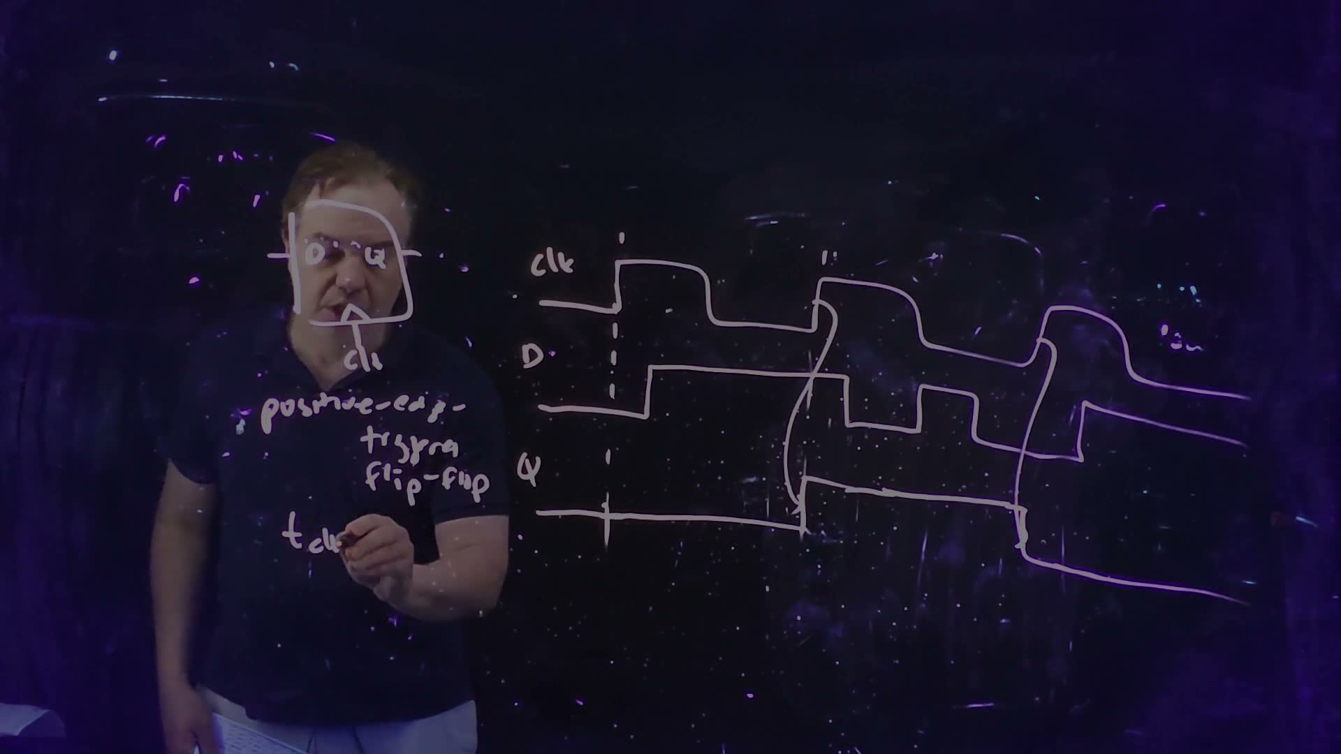
Fair copy of the board above (Lecture12 @ 52:26), mark for mark in its own layout. The board is in one pen (the pale orange one) and is copied in black. The waveform rows slope down to the right on the board and are levelled, with every edge set vertical; the board draws Q’s two edges a little left of the clock edges their arrows come from, and the copy puts them just after, as the lecturer narrates. “t_clk” at the lower left is being written; it reads “t_clk-Q ⇒ clock-to-Q” at 52:52.

Lecture12 @ 52:52Setup and hold around the rising (active) edge.

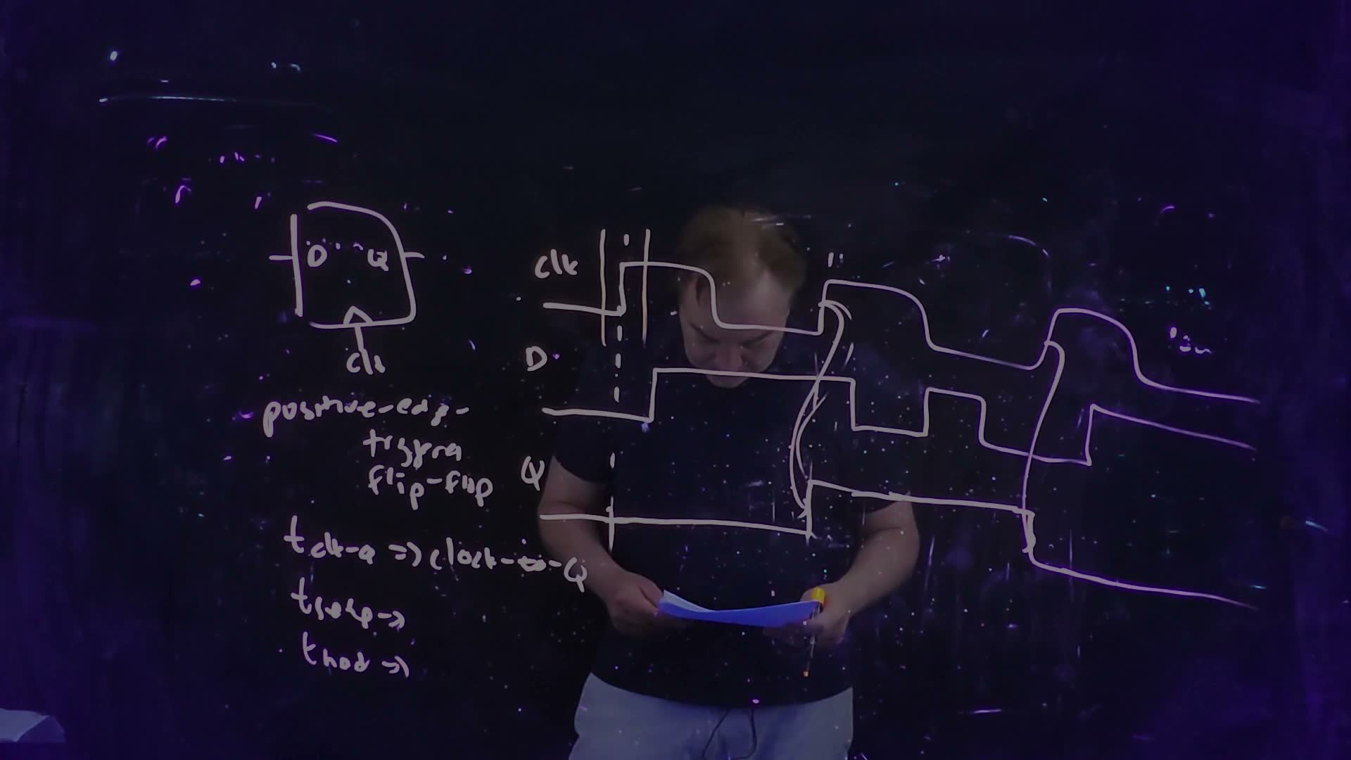
Fair copy of the board above (Lecture12 @ 52:52), mark for mark in its own layout, in black (one pen, the pale orange one). New since 52:26 are the two vertical lines either side of the first rising edge, for setup (before) and hold (after), and the three parameters at the lower left. The lines are solid on the board; the dashed one between them is 52:26’s. The rows are levelled and Q’s edges set just after the clock edges, as in the 52:26 copy.

Reading the board's flip-flop (board, 51:50–52:16)

1. Start with Q = 0 (51:51).
2. Edge 1: D is 0, so Q stays 0. D rises soon after; the flip-flop does not care.
3. Edge 2: D is 1, so Q rises a little after the edge. D then falls, rises and falls again before edge 3; Q ignores all of it.
4. Edge 3: D is 0, so Q falls. D rises just after; Q holds 0 until the next edge.

Every Q edge is caused by a clock edge, so a flip-flop has only one delay, $t_{clk\to Q}$ (52:21) board. There is no $t_{D\to Q}$tD→Q​: D never passes straight through. Setup and hold sit around the active edge, the rising edge here, because that is the moment the flip-flop decides what to keep; the aperture is $t_{setup} + t_{hold}$thold​, as for a latch (52:37–53:18) board.

The edge-triggered flip-flopboard

$$Q(t_e + t_{clk\to Q}) = D(t_e)$$

Holds when: D steady from t_setup before to t_hold after each active edge t_e (rising for a positive-edge flip-flop)

Latch against flip-flop on the same inputs

added Feed the shared stimulus to a positive-edge flip-flop.

The positive-edge flip-flop on the shared stimulus (added numbers)

1. The samples. At the rising edges 2, 12, 22 and 32 ns, D is 1, 0, 1 and 1.
2. 2 ns: D = 1, Q = 0, so Q rises at $2 + 0.3 = 2.3$ ns.
3. 12 ns: D = 0, so Q falls at 12.3 ns.
4. 22 ns: D = 1, so Q rises at 22.3 ns.
5. 32 ns: D = 1 = Q, so nothing happens.
6. The windows. No D edge lies within $[t - 0.4,\ t + 0.2]$ ns of a rising edge $t$t: the closest any comes is D’s fall at 3.5 ns, 1.5 ns after the edge at 2 ns. Every sample is certain.

A latch and a flip-flop on the same inputs added, computed from the shared stimulus with $t_{clk\to Q} = 0.3$ ns. The transparent-high latch’s output $Q_{latch}$ follows D through each high phase (eight edges). The positive-edge flip-flop’s output $Q_{FF}$ changes only just after a rising edge (dotted), to the value D had at that edge: three edges, and none at 32 ns, where D already equals Q.

The transparent-high latch of Section 2 gave Q eight edges on these inputs; the flip-flop gives three. Its output is a clean copy of D sampled once per cycle, delayed by $t_{clk\to Q}$tclk→Q​. The flip-flop’s edges at 2.3, 12.3 and 22.3 ns coincide with three of the latch’s clock-caused edges, ①, ④ and ⑤. Every other difference traces back to D moving during a high phase: the latch’s data-caused edges, and ⑦, which only restores the 1 the latch lost at ⑥.

The overhead every cycle pays

A flip-flop costs time twice in every cycle (53:27) board: the data it launches leaves only $t_{clk\to Q}$ after the edge, and the data it captures must arrive $t_{setup}$ before the edge. Together they are the latch overhead, “the time … that we waste, that we give up in our flop-based design from our ability to do actual logic in a cycle” (53:27). The lecture uses the name “latch overhead” for flip-flops too.

The board (Lecture12 @ 54:21)

Lecture12 @ 54:21't_clk→q + t_setup = latch overhead'.

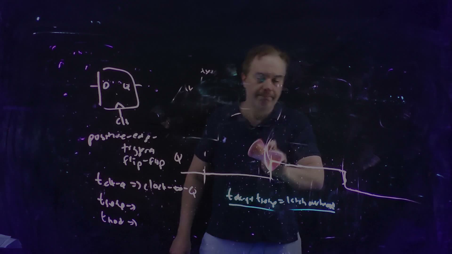
Fair copy of the board above (Lecture12 @ 54:21), mark for mark in its own layout, in black (the pale orange pen, and the cyan one for the new line and its underline). The lecturer is wiping the flip-flop waveforms (“so let me erase this”, 53:58–54:31): the copy keeps what still stands, Q’s row, the end of the first curved arrow and two pieces of the dashed line, and leaves out the scraps and ghosts of the rest; the eraser in his hand covers the middle. New since 52:52 is the underlined line “t_clk-q + t_setup = latch overhead”. The rows are levelled as in the 52:26 copy.

Latch overheadboard

$$\text{overhead} = t_{clk\to Q} + t_{setup}$$

Holds when: per cycle, for a flop-based design: the launching flip-flop's clock-to-Q plus the capturing flip-flop's setup

Memorize or derive. Memorize both boxes: Q takes D at the active edge, after $t_{clk\to Q}$tclk→Q​; the overhead is $t_{clk\to Q} + t_{setup}$tsetup​. On the shared stimulus it is $0.3 + 0.4 = 0.7$ ns.

Flop-based design, and the lecturer’s dissent

Most standard-cell ASIC designs are flop-based: every storage element is a flip-flop on one clock, because the timing constraints are much easier to analyse (48:42–49:04, paraphrased). The lecturer disagrees with the habit: “flop-based design is not the best design style to use”, and “we should be doing latch-based design” (49:17, 49:40). Chapter 14 makes his case: latches can lend unused time from one stage to the next (time borrowing) and tolerate clock skew, which flip-flops cannot.

Traps.

• Redundant names. “Edge-triggered flip-flop” and “level-sensitive latch” say the same thing twice, and “latch” is often said for a flip-flop (50:42). Look for the caret.
• A $t_{D\to Q}$ for a flip-flop. It has none. FN17-5 gives its latches a $t_{d-q}$td−q​, but a path from flip-flop to flip-flop never uses it (Section 10).
• Q following D between edges. Only a latch does that.

Check yourself The shared stimulus goes into a negative-edge flip-flop (t_clk→Q = 0.3 ns, Q = 0 at the start). What does it sample, and when does Q change?

A negative-edge flip-flop samples at the falling edges, 7, 17, 27 and 37 ns, where D is 1 (it rose at 5), 0 (fell at 9), 0 (fell at 24) and 0 (fell at 34). So Q rises at $7 + 0.3 = 7.3$ ns and falls at 17.3 ns, and then nothing more: the samples at 27 and 37 ns equal Q. Section 10 builds exactly this flip-flop from two latches.

Check yourself A flip-flop has t_clk→Q = 60 ps and t_setup = 40 ps. What fraction of a 1 ns cycle is overhead?

Overhead $= 60 + 40 = 100$ ps, which is 10% of 1000 ps. The logic gets the other 900 ps.

10. Master–slave: a flip-flop from two latches

You need

Two latch polarities (Section 2). A transparent-high latch is open while clk = 1 and closes at the falling edge; a transparent-low latch (a latch on $\overline{\text{clk}}$clk, or with a bubble on clk) is open while clk = 0 and closes at the rising edge.

The window (Section 3). What a latch keeps is D at its closing edge, protected by $t_{setup}$ before and $t_{hold}$ after it.

The setup–hold window around a latch’s closing edge $t_c$ (Lecture12 @ 36:53, redrawn). Original figure ↑

What a flip-flop does (Section 9). It samples D at its active edge and shows it after $t_{clk\to Q}$tclk→Q​, holding in between.

The positive-edge flip-flop (Lecture12 @ 52:26, redrawn): Q changes only just after a rising edge, to the value D had at that edge. Original figure ↑

The question. Section 9 drew the flip-flop as a box with a caret. What is inside it, and where do its setup time, hold time and clock-to-Q delay come from?

Two latches on opposite phases

Put two latches in series (54:31–54:58) board: the master on clk (transparent high), then the slave on $\overline{\text{clk}}$ (transparent while clk = 0). The master’s output, here called $Q_M$QM​, is the slave’s D. (This term’s class noted IBM’s names for the two, L1 and L2 added.)

A master–slave flip-flop (redrawn from the board, Lecture12 @ 56:32). The master latch is transparent while clk = 1 and the slave while clk = 0, so the pair captures D at each falling edge of clk (dotted lines): a negative-edge flip-flop, drawn at the left with a caret and a bubble on its clock. Its setup and hold times belong to the master, which closes at that edge; its clock-to-Q delay belongs to the slave, which opens then.

The board (Lecture12 @ 56:32)

Lecture12 @ 56:32Master on clk, slave on clk-bar: a negative-edge flip-flop (bubble added on the symbol); setup and hold from the master, clock-to-Q from the slave.

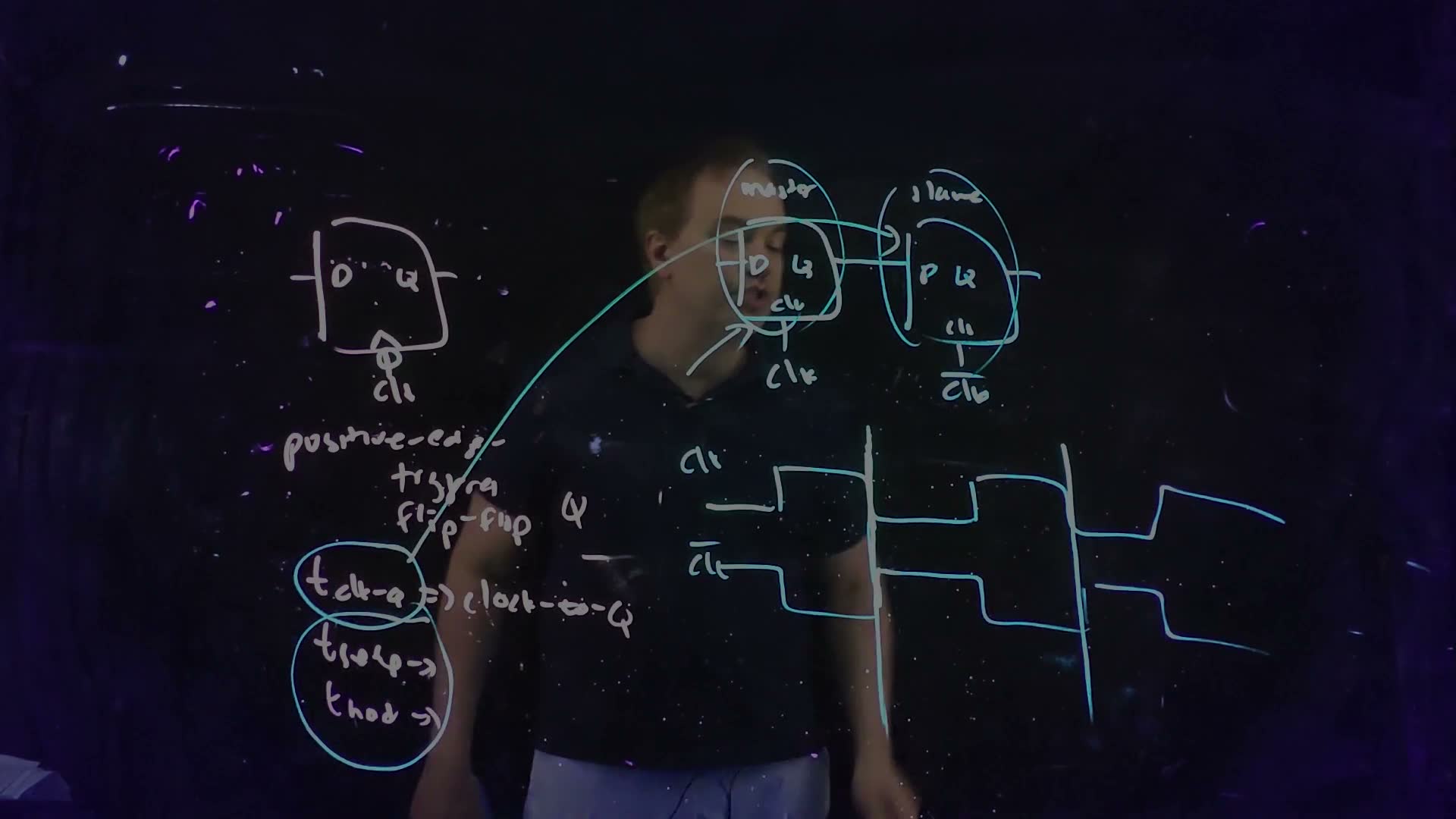
Fair copy of the board above (Lecture12 @ 56:32), mark for mark in its own layout, in black (the pale orange pen for the flip-flop at the left, the cyan pen for everything added since 54:21). The bubble under the caret makes the symbol a negative-edge flip-flop, as the master–slave pair is (55:52–56:17); the words beside it still read “positive-edge-triggered”. The arrow onto the master’s clock input starts behind the lecturer, and the board is wiped before he moves (58:58), so its start is not restored; the narration ties it to the circled setup and hold (56:17). The waveform rows are levelled and the edges set vertical: clk’s falls, clk-bar’s rises and the two long lines coincide, as on the board.

Following one cycle (board, 54:58–55:51)

1. clk = 1. The master is transparent: $Q_M$ follows D. The slave is opaque: Q holds its old value, whatever $Q_M$ does.
2. clk falls. The master closes and keeps D’s value at that edge; “at exactly that same point, the slave opens” (55:27), and Q takes $Q_M$QM​.
3. clk = 0. The master is opaque, so $Q_M$ is frozen. The slave is open, but its input is not moving, so Q stays steady.
4. clk rises. The slave closes, holding Q, just as the master opens to follow D again. Q does not change.
5. So Q changes only just after clk falls, to the value D had at that falling edge: “this acts like a negative edge-triggered flip-flop” (55:51). The board then adds a bubble under the caret of its flip-flop symbol board.

At no moment are both latches open, so D can never run straight through to Q: that is what makes the pair edge-triggered.

Where its parameters come from

“The setup and hold time of this flip-flop are … determined by the setup and hold time of the master latch. The clock-to-Q delay … by the clock-to-Q delay of … the slave latch” (56:17) board. Both follow from step 2. The decision about what to keep is made when the master closes, so its window is the flip-flop’s window. The new Q appears when the slave opens on a $Q_M$ that is already settled, so it is the slave’s clock-to-Q delay.

Master–slave flip-flopboard

$$t_{setup,FF} = t_{setup,\,master}, \qquad t_{hold,FF} = t_{hold,\,master}$$$$t_{clk\to Q,FF} = t_{clk\to Q,\,slave}$$

Holds when: clk and clk̄ exactly complementary (if they overlap, both latches are open at once and data can race through: Chapter 14); the active edge is the master's closing edge

Memorize or derive. Memorize the three parameters. Derive the active edge rather than memorizing it: it is the edge at which the master closes (steps 1–5). A transparent-high master closes at the falling edge, so the flip-flop is negative-edge; swap the phases and it becomes positive-edge.

“Nearly all flip-flops are created” this way (56:39). The lecture mentions “one other way to make a latch look like a flip-flop”, used in some high-performance processors (56:52, paraphrased): the pulsed latch, which Chapter 14 teaches.

A worked example: the shared stimulus through the pair

added Both latches have $t_{clk\to Q} = 0.3$ ns and $t_{D\to Q} = 0.2$ ns; the master has $t_{setup} = 0.4$ ns and $t_{hold} = 0.2$ ns. The stimulus is Section 2’s: clk high on [2, 7), [12, 17), [22, 27), [32, 37) ns; D = 1 at 0 with edges at 3.5↓, 5↑, 9↓, 19↑, 24↓, 29↑, 34↓ ns; both outputs start at 0.

Master, then slave (added numbers)

1. The master is Section 2’s latch, on the same clock and the same D, so $Q_M$ is exactly Section 2’s output: 2.3↑, 3.7↓, 5.2↑, 12.3↓, 22.3↑, 24.2↓, 32.3↑, 34.2↓ ns. Every one of those edges falls while clk = 1, when the slave is closed.
2. 7 ns, clk falls. The slave opens on $Q_M = 1$ while Q = 0: Q rises at $7 + 0.3 = 7.3$ ns.
3. 17 ns. $Q_M = 0$ (it fell at 12.3): Q falls at 17.3 ns.
4. 27 ns. $Q_M = 0$ (it fell at 24.2) $= Q$Q: nothing happens.
5. 37 ns. $Q_M = 0$ (it fell at 34.2) $= Q$Q: nothing happens.
6. The result. Q has two edges, 7.3↑ and 17.3↓, and D’s samples at the falling edges are 1, 0, 0, 0. D’s two later high pulses, 19–24 ns and 29–34 ns, never reach Q. Each rises while clk = 0, when the master is closed, so the master sees only its tail inside the next high phase ($Q_M$QM​ 22.3↑ to 24.2↓, and 32.3↑ to 34.2↓). D has fallen again before the master closes at 27 and 37 ns, so the slave opens on $Q_M = 0$ both times.

The shared stimulus through a master–slave pair added, computed with $t_{clk\to Q} = 0.3$ ns and $t_{D\to Q} = 0.2$ ns. The master is transparent while clk = 1 (shaded), so $Q_M$ follows D in each high phase. The slave is transparent while clk = 0 and copies $Q_M$QM​, which is then frozen, so Q changes only just after the falling edges of clk (dotted), at 7.3 and 17.3 ns. At 27 and 37 ns, $Q_M = 0 = Q$ and nothing changes.

Check. Section 9’s check fed the same stimulus to a negative-edge flip-flop and got 7.3↑ and 17.3↓: the same edges. The flip-flop built here has $t_{setup} = 0.4$ ns and $t_{hold} = 0.2$ ns from its master and $t_{clk\to Q} = 0.3$ ns from its slave.

Reading an exam’s latch pair

added Past finals draw flip-flops as their latches. FN17-5 shows four latches in a row on clocks $\phi_1$ϕ1​, $\phi_2$ϕ2​, $\phi_1'$ and $\phi_2'$ with the logic between the second and third. Read them in pairs: a latch on $\phi_1$ followed by a latch on $\phi_2 = \overline{\phi_1}$ is one master–slave flip-flop, so the figure is two flip-flops with logic between them, the long path of Section 11. Find each flip-flop’s active edge from its master: the edge at which the master’s clock closes it. The flip-flop then takes its setup time from the first latch of the pair and its clock-to-Q from the second, and the latches’ $t_{d-q}$ plays no part in a flip-flop-to-flip-flop path.

Traps.

• “Positive-edge, because the master is transparent high.” The master is open while clk is high and closes when it falls: negative-edge.
• $t_{clk\to Q}$ from the master. The new Q appears when the slave opens; the master’s delay only has to be over before then.
• Four latches, four stages. FN17-5’s four latches are two flip-flops: one path, one constraint.
• Overlapping clocks. With clk and $\overline{\text{clk}}$ overlapping, both latches are briefly open and data can race through (Chapter 14).

Check yourself Build the pair the other way: master transparent-low (open while clk = 0), slave transparent-high. Which edge is active, and what does Q do on the shared stimulus?

The master closes when clk rises, so the flip-flop is positive-edge. The master (open on [0, 2), [7, 12), …) follows D while clk is low; at each rising edge the slave opens on the master’s value. The samples at 2, 12, 22 and 32 ns are 1, 0, 1, 1, so Q rises at 2.3 ns, falls at 12.3 ns, rises at 22.3 ns, and stays at 32 ns: Section 9’s positive-edge flip-flop exactly.

Check yourself Each latch of a pair has t_setup = 5 ps, t_clk→Q = 10 ps and t_D→Q = 10 ps (FN17-5's values). What are the flip-flop's setup time and clock-to-Q delay?

Setup from the master, 5 ps; clock-to-Q from the slave, 10 ps. The $t_{D\to Q}$ of 10 ps does not appear: inside a master–slave pair the slave is closed whenever $Q_M$ moves.

11. The long path: how fast can the clock run?

You need

A flip-flop’s parameters (Sections 9–10). Q takes D at the active edge, $t_{clk\to Q}$ later; D must be steady from $t_{setup}$ before to $t_{hold}$ after that edge; the latch overhead is $t_{clk\to Q} + t_{setup}$tsetup​.

The master–slave flip-flop (Lecture12 @ 56:32, redrawn): setup and hold from the master, clock-to-Q from the slave. Original figure ↑

A path’s delay (Chapter 8). The logic between two flip-flops is a path of gates with delay $\tau_{inv}\sum g_ih_i$τinv​∑gi​hi​, where $\tau_{inv}$ is the fan-out-of-one inverter delay. The course’s yardstick is the FO4 delay, an inverter driving four copies of itself: a gain of 4, so $4\tau_{inv}$ (Chapter 7).

Process corners (Chapter 6 §8). SS is the corner with slow NFETs and slow PFETs; with the lowest supply and the highest temperature it gives the slowest gates.

The question. In a flop-based design, how much logic fits between two flip-flops for a given clock, or, turned around, how fast can the clock run for a given amount of logic?

Launch, logic, capture

The board’s setting (57:07–57:51) board: a flip-flop, some combinational logic, another flip-flop, both on the same clock, edge-triggered on its rising edge. “What is the longest path that I can have here in this combinational logic and have this still … function?” (58:02).

The long path (redrawn from the board, Lecture12 @ 61:43). Data launched at one rising edge of clk must pass the launching flip-flop ($t_{clk\to Q}$tclk→Q​) and the logic ($t_{logic}$tlogic​) and still arrive $t_{setup}$ before the next rising edge, one period $T_{cycle}$ later: $t_{clk\to Q} + t_{logic} + t_{setup} \le T_{cycle}$Tcycle​. The board draws the equality case, $t_{setup}$ ending exactly at the capture edge.

The board (Lecture12 @ 61:43)

Lecture12 @ 61:43Long-path analysis: the inequality, the overhead, and late mode at the PVT corner SS, lowest voltage, highest temperature.

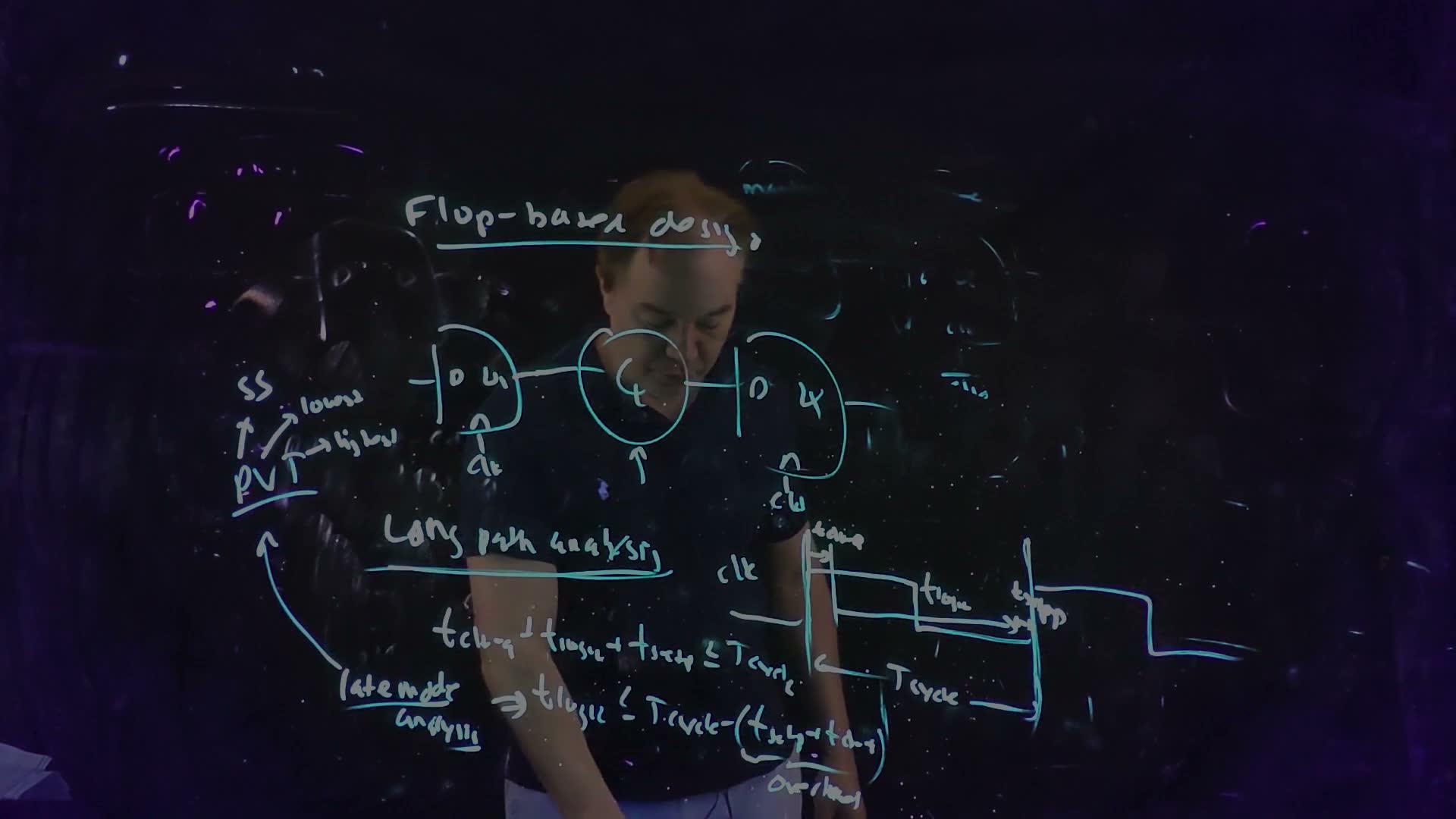
Fair copy of the board above (Lecture12 @ 61:43), mark for mark in its own layout, in black (one pen, the cyan one). The logic circle’s label, a C with a crossed L, is set as CL (combinational logic, 57:43). Nothing is hidden: the ink stays visible over the lecturer. The clock is levelled with its edges set vertical, the long lines on its rising edges as on the board, and the T_cycle and t_logic arrows are levelled with it. Faint remains of the earlier boards are left out.

Adding up one cycle (board, 58:21–59:35)

1. Launch. At a rising edge the first flip-flop takes its D. Its new Q is valid $t_{clk\to Q}$ later.
2. Logic. The new value runs through the logic; along its longest path it arrives at the second flip-flop’s D another $t_{logic}$ later.
3. Capture. The second flip-flop samples at the next rising edge, $T_{cycle}$ after the launch, and needs its D steady $t_{setup}$ before that edge.
4. So the three must fit in a cycle: $t_{clk\to Q} + t_{logic} + t_{setup} \le T_{cycle}$ board.
5. Solve for the logic: $t_{logic} \le T_{cycle} - (t_{setup} + t_{clk\to Q})$ board. The bracket is the latch overhead of Section 9, which the board labels “overhead”.

The long-path (setup) constraintboard

$$t_{clk\to Q} + t_{logic} + t_{setup} \le T_{cycle}$$$$t_{logic} \le T_{cycle} - \left(t_{setup} + t_{clk\to Q}\right)$$

Holds when: zero clock skew (both flip-flops see the edge at the same time); a single-cycle path between flip-flops on the same edge; the launching flip-flop's t_clk→Q, the capturing one's t_setup; maximum delays, at the slow corner

The fastest clock follows by turning the inequality around added: with a longest logic path $t_{logic,max}$tlogic,max​, the period must be at least the sum, so

$$f_{clk,max} = \frac{1}{t_{clk\to Q} + t_{logic,max} + t_{setup}}$$

Memorize or derive. Memorize the first inequality and its conditions. Derive the other two in one line each: subtract the overhead for $t_{logic}$tlogic​; invert the sum for $f_{clk,max}$fclk,max​.

Late mode: check it at the slowest corner

This check is long-path or late-mode analysis (59:45) board: it fails when signals arrive too late. So it is checked where everything is slowest: “my slow-slow corner for my process … the lowest available voltage … the highest possible temperature” (60:21–60:50), the board’s “PVT → SS, lowest, highest”.

The board (Lecture12 @ 60:58)

Lecture12 @ 60:58Late-mode analysis at the PVT corner: SS process, lowest voltage, highest temperature.

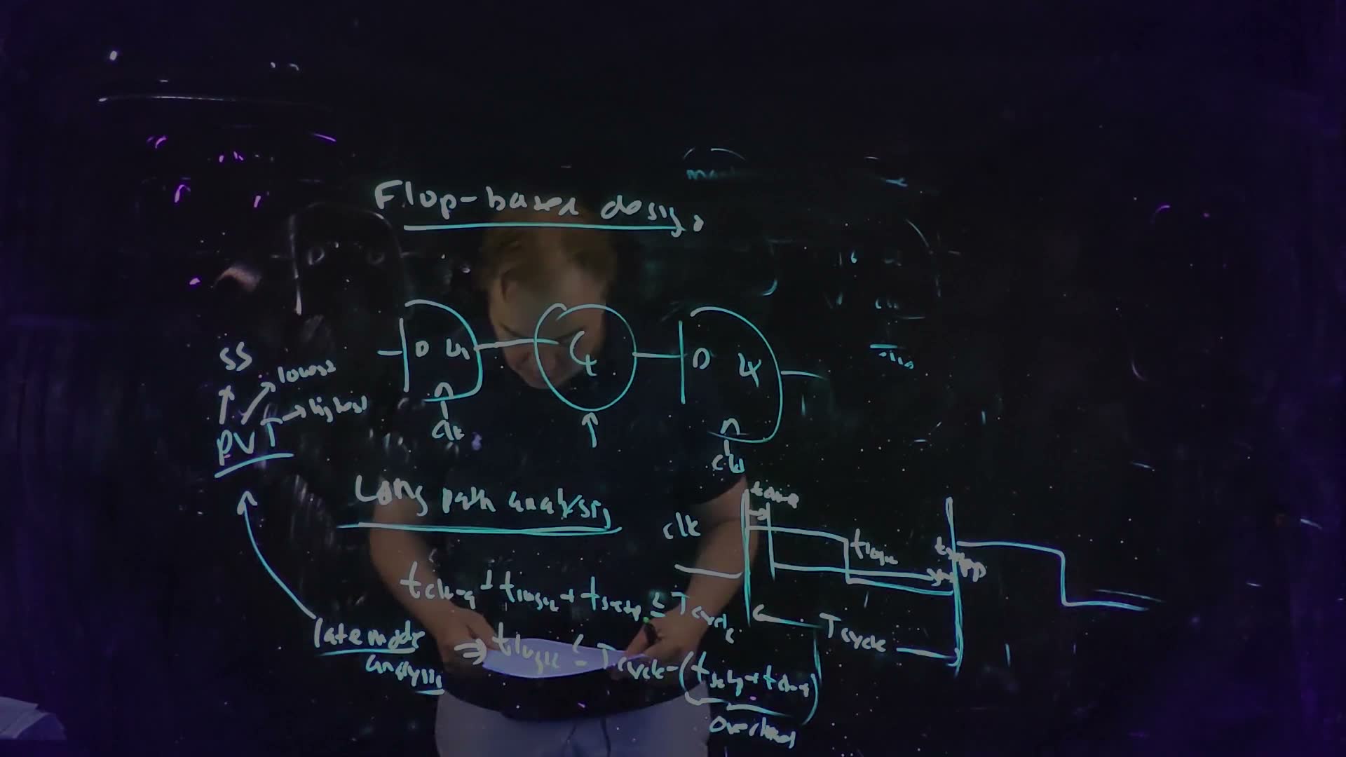
Fair copy of the board above (Lecture12 @ 60:58), mark for mark in its own layout, in black (one pen, the cyan one). The board is finished here: “PVT” and its three corners went up as he named them (60:25), and nothing is added before the lecture ends, so the copy is the one under the 61:43 frame. The sheet of notes in the lecturer’s hands lies over “t_logic ≤ T” of the second inequality, but the ink reads through it; nothing is restored. The clock is levelled with its edges set vertical, as there.

If a path fails, the remedy is always available: slow the clock. A larger $T_{cycle}$ fixes any long-path failure. The overhead, though, is paid in every cycle by every stage, so cutting a path into more pipeline stages buys a faster clock but spends a larger share of each cycle on overhead.

A worked example: 15 FO4

This term’s class gave typical numbers added (Fall 2026 Lecture 11, 1:11:45): “The cycle time might be 15 FO4s. Three of them would be latch overhead … I got 12 FO4s to do logic.” Turn them into picoseconds with the course’s FO4 $= 4\tau_{inv}$ and, for example, $\tau_{inv} = 10$ ps.

One cycle’s budget added, computed from $T_{cycle} = 600$ ps (15 FO4, with FO4 $= 4\tau_{inv} = 40$ ps), $t_{clk\to Q} = 80$ ps and $t_{setup} = 40$ ps. The overhead, $t_{clk\to Q} + t_{setup} = 120$ ps (3 FO4), comes off every cycle and leaves $t_{logic} \le 480$ ps, 12 FO4, for the logic. The axis is in ps (ticks every FO4) and, below, in FO4.

The budget of one cycle (added conversion of the class's numbers)

1. The yardstick. FO4 $= 4 \times 10 = 40$ ps.
2. The cycle. $T_{cycle} = 15 \times 40 = 600$ ps, so $f_{clk} = 1/600\ \text{ps} = 1.67$ GHz.
3. The overhead. Take $t_{clk\to Q} = 80$ ps and $t_{setup} = 40$ ps: $120$ ps, which is 3 FO4, 20% of the cycle.
4. The logic budget. $t_{logic} \le 600 - (40 + 80) = 480$ ps $= 48\,\tau_{inv} = 12$ FO4.
5. Does a path fit? A path of six stages, each with gain 4 (Chapter 8), takes $6 \times 4 = 24\,\tau_{inv} = 240$ ps. It fits, with 240 ps to spare.
6. The fastest clock for a longer path. A 520 ps path needs $T_{cycle} \ge 80 + 520 + 40 = 640$ ps, so $f_{clk,max} = 1/640\ \text{ps} = 1.5625$ GHz.

Check. In FO4 units the budget is $15 - 3 = 12$ FO4, the class’s own figure, and $12 \times 40 = 480$ ps matches step 4.

What a slower clock cannot fix (a preview)

added The lecture ends by announcing “a little more subtle one, which is the short path analysis”, and clock skew: “Right now I’m assuming that these clocks are arriving at exactly the same time” (60:58–61:28). Chapter 14 teaches both; here is what they are, in one paragraph. The long path asks whether new data arrives before the next edge’s setup window. The short path asks whether new data, launched at an edge, arrives so early that it reaches the capturing flip-flop within the hold time of the same edge and overwrites the value being captured. With zero skew that needs $t_{clk\to Q} + t_{logic,min} \ge t_{hold}$thold​. $T_{cycle}$ does not appear in it, so a slower clock can never fix a short-path failure; only adding delay to the short paths can. Skew, clocks that do not arrive at both flip-flops at once, enters both constraints, and Chapter 14 shows with which sign.

Traps.

• $t_{hold}$ in the long path. Hold belongs to the short path. The long path uses $t_{clk\to Q}$ and $t_{setup}$ only.
• Mixing up the two flip-flops. It is the launching flip-flop’s $t_{clk\to Q}$ and the capturing one’s $t_{setup}$tsetup​.
• Checking at the fast corner. Late mode needs the slowest gates: SS, lowest voltage, highest temperature.
• “Deeper pipelining is free.” Each stage pays the overhead again.
• The name. The lecture says “latch overhead” even for flip-flops; it is still $t_{clk\to Q} + t_{setup}$tsetup​.

Check yourself In the 15 FO4 example (T_cycle = 600 ps, t_clk→Q = 80 ps, t_setup = 40 ps), the capturing flip-flop's clock arrives 30 ps early. What is the largest t_logic now?

The capture edge comes 30 ps sooner, so the data has 30 ps less time to arrive before its setup window: $t_{logic} \le 600 - 120 - 30 = 450$ ps. (An early capture clock hurts the long path; Chapter 14 shows why a late one hurts the short path instead.)

Check yourself The 520 ps path is split into two pipeline stages of 260 ps each, with the same flip-flops. What is the new fastest clock, and what share of each cycle is overhead?

Each stage needs $80 + 260 + 40 = 380$ ps, so $f_{clk,max} = 1/380\ \text{ps} = 2.63$ GHz, up from 1.56 GHz. But the 120 ps overhead is now $120/380 = 32\%$ of the cycle, against $120/640 \approx 19\%$ before: the second stage paid the overhead again.

Check yourself Why can a clock edge that reaches the capturing flip-flop later than the launching one cause a failure that no clock period fixes?

The launching flip-flop releases new data at its edge, and through a short path it can reach the capturing flip-flop while that flip-flop is still holding on to the same edge (its edge is late, so its hold window is late too). The new data then overwrites the value being captured. Nothing in that race involves $T_{cycle}$Tcycle​, so slowing the clock does not help; the designer must make the short paths longer. FN10-6d asks exactly this, with jitter as the cause; Chapter 14 teaches the constraint, and the practice page fs1 solves the part.

On the exam

Storage elements and flop-based timing are on all four past finals: FN19-9 (the unwritable latch, 10 points), FN17-5 (two flip-flops built from latches, 40 points over four parts) and FN10-6d (7 points) are mapped below, and FN12-7b (flip-flop skew) is Chapter 14’s. No past part is solved on this page. The practice pages for the sequential group, fs1 (flip-flop and latch timing) and fs2 (clock generation and storage cells), solve them, and Chapter 14 (Lecture 13) adds the short path and skew that FN17-5 and FN10-6d also need.

Section	Past-paper parts (points)	What they ask
§6 latch circuits; §7 the write fight; §8 gated feedback	FN19-9 (10), on fs2	“He finds that he is unable to write the latch … What has gone wrong? How can this be fixed?”: name the fight (§7), say which direction is worse, fix it by weakening the feedback or, best, by gating it (§8)
§10 master–slave	FN17-5a (10), on fs1, with Chapter 14	read each $\phi_1$/$\phi_2$ latch pair as one flip-flop, then ask whether the primed clocks’ 50 ps skew breaks it
§10 master–slave; §11 the long path	FN17-5b (10), on fs1, with Chapter 14	the largest $t_{logic}$tlogic​: the long path with the pairs’ setup and clock-to-Q, less the skew; the latches’ $t_{d-q}$ is not used
§10, §11	FN17-5c–d (20), on fs1, with Chapter 14	fixing the clocks if (a) fails, and the new largest $t_{logic}$
§9 flip-flop parameters; §11 the preview	FN10-6d (7), on fs1, with Chapter 14	whether clock jitter can cause a failure no clock period fixes: the short path, whose constraint has no $T_{cycle}$
§1–§5	none directly	background for every sequential question: the vocabulary, the window, metastability

Leaning on this chapter. FN12-7b (flip-flop skew), FN19-5a (hold on a pulsed latch) and PS5-Q1 (latch timing) are taught in Chapter 14, but read their circuits with §2, §3, §9 and §10. Chapter 19’s SRAM cell builds on §5’s butterfly and §7’s write fight.

Memorize.

• A transparent-high latch follows D while clk = 1 and holds D’s value at the falling (closing) edge; a bubble swaps the levels. A D edge through an open latch takes $t_{D\to Q}$tD→Q​; an opening edge on a D that differs from Q takes $t_{clk\to Q}$ (§2).
• D must be steady on $[t_c - t_{setup},\ t_c + t_{hold}]$ around the closing edge of a latch, or the active edge of a flip-flop; the aperture is $t_{setup} + t_{hold}$ (§3, §9).
• Static storage is a cross-coupled inverter pair (SRAM); dynamic storage is charge on a node (DRAM, refresh). The butterfly diagram has two stable points and a metastable one in the middle (§4, §5).
• The static latch: pass NFET on clk, forward inverter, always-on feedback inverter; output $\overline{Q}$Q​. To write it, the write path must overpower the feedback device; writing a 1 through an NFET is the harder direction (§6, §7).
• The standard-cell latch gates its feedback on $\overline{\text{clk}}$clk, with transmission gates on both switches (§8).
• A flip-flop: $Q(t_e + t_{clk\to Q}) = D(t_e)$ at its active edge; no $t_{D\to Q}$tD→Q​. Latch overhead $= t_{clk\to Q} + t_{setup}$ (§9).
• Master on clk, slave on $\overline{\text{clk}}$clk: a negative-edge flip-flop. Setup and hold from the master, clock-to-Q from the slave (§10).
• $t_{clk\to Q} + t_{logic} + t_{setup} \le T_{cycle}$Tcycle​, with zero skew, checked at the slow corner (SS, lowest $V_{DD}$VDD​, highest temperature) (§11).

Derive (each in a line or three).

• The largest logic delay and the fastest clock. Subtract the overhead: $t_{logic} \le T_{cycle} - (t_{setup} + t_{clk\to Q})$tclk→Q​). Invert the sum: $f_{clk,max} = 1/(t_{clk\to Q} + t_{logic,max} + t_{setup})$ (§11).
• A latch pair’s active edge. Follow one cycle: the flip-flop decides when the master closes, so a master on clk (transparent high) gives a falling-edge flip-flop (§10).
• The write fight, roughly. Series resistances add. Writing a 0: $R_{down} = R/W_{drv} + R/W_{pass}$ against the feedback PFET’s $R_{up} = 2R/W_{fb}$2R/Wfb​, then the divider $V_X = V_{DD}R_{down}/(R_{down} + R_{up})$Rup​), writable if $V_X < V_M$VM​. Writing a 1: $R_{up} = 2R/W_{drv} + 2R/W_{pass}$ (driver PFET, pass NFET pulling up) against the feedback NFET’s $R_{down} = R/W_{fb}$R/Wfb​, writable if $V_X > V_M$ (§7, added).
• Retention of a dynamic node. $I = C\,dV/dt$ with a constant leak: $t_{ret} = C_X\,\Delta V/I_{leak}$ (§4, added).
• Why the middle of the butterfly is unstable. A nudge $\delta$ becomes $A_AA_B\,\delta$ after one trip around the loop; at the middle the loop gain exceeds 1 (§5, added).

Method cards. The playbook’s cards for this chapter’s families are not written yet. Two families will cover these parts: the latch-writability card (FN19-9: name the fight, estimate it, fix it two ways) and the flip-flop timing card (FN17-5, FN10-6d: find the flip-flops, then the long path, then the short path).

Formulas to remember

Formula	Meaning
clk = 1: Q follows D after $t_{D\to Q}$tD→Q​; opening on $D \ne Q$Q: after $t_{clk\to Q}$tclk→Q​; clk = 0: $Q = D(t_c)$	the transparent-high D latch
D steady on $[t_c - t_{setup},\ t_c + t_{hold}]$thold​]; aperture $t_{setup} + t_{hold}$	the window, around the closing (latch) or active (flip-flop) edge
$t_{ret} \approx C_X\,\Delta V/I_{leak}$	how long a dynamic node holds a bit (added)
$V_2 = f(V_1)$ and $V_1 = f(V_2)$f(V2​); three crossings	the butterfly: two stable states, one metastable
loop gain $A_AA_B > 1$ at the middle	why the middle state does not hold (added illustration)
$V_X \approx V_{DD}R_{down}/(R_{down} + R_{up})$Rup​); writable if $V_X < V_M$	the write fight as a divider (added, rough)
feedback gated on $\overline{\text{clk}}$clk, transmission gates	the standard-cell latch: no fight
$Q(t_e + t_{clk\to Q}) = D(t_e)$	the edge-triggered flip-flop
overhead $= t_{clk\to Q} + t_{setup}$	the latch overhead of every flop-based cycle
master on clk, slave on $\overline{\text{clk}}$ ⇒ negative edge; setup, hold: master; $t_{clk\to Q}$tclk→Q​: slave	the master–slave flip-flop
$t_{clk\to Q} + t_{logic} + t_{setup} \le T_{cycle}$	the long path (late mode, slow corner, zero skew)
$f_{clk,max} = 1/(t_{clk\to Q} + t_{logic,max} + t_{setup})$	the fastest clock (added)
$t_{clk\to Q} + t_{logic,min} \ge t_{hold}$	the short path, zero skew (preview; Chapter 14)

The lecture’s boards

All the boards of Lecture 12 from 23:15 (14 frames)

Lecture12 @ 28:52 synchronous, asynchronous; latch ⇒ levels, flip-flop ⇒ edges

Lecture12 @ 31:03 the D latch, transparent high: clk and D

Lecture12 @ 36:53 Q traced; t_D→Q, t_clk→Q; setup and hold

Lecture12 @ 39:40 memory: static (the loop), dynamic

Lecture12 @ 41:40 the butterfly: stable and metastable points

Lecture12 @ 44:46 the static and the dynamic D latch

Lecture12 @ 46:54 the write fight; writeability

Lecture12 @ 48:35 gated feedback with transmission gates

Lecture12 @ 52:26 the positive-edge flip-flop

Lecture12 @ 52:52 setup and hold around the rising edge

Lecture12 @ 54:21 t_clk→q + t_setup = latch overhead

Lecture12 @ 56:32 master–slave: a negative-edge flip-flop

Lecture12 @ 60:58 late mode: PVT → SS, lowest, highest

Lecture12 @ 61:43 long path: t_logic ≤ T_cycle − overhead