9. Fabrication and layout

So far every circuit in this guide has been a schematic: transistor symbols joined by wires. A foundry can’t build a schematic. It builds whatever shapes you draw, layer by layer, on the wafer. Lecture 9 is about those shapes: the layout. It names the layers of the class’s IBM 90 nm technology and what each one makes, shows them in cross-section, explains the rules the drawing must obey and the tools that check it, and then lays out an inverter on the board. It ends with the stick diagram, a quick sketch of a layout that the next lecture, and two past midterms, use.

This lecture has no derivations. What it gives you is a vocabulary and a set of rules for reading a drawing; the chapter adds worked readings and practice in the exam’s form.

After this chapter you can:

1. explain how a layout becomes masks, what GDS and tape-out are, and what FEOL and BEOL mean;
2. say what each front-end layer (RX, NW, PC, BP, CA) makes, and use reverse toning to tell n+ from p+ and a transistor from a tie;
3. describe the class’s 5-2-2 metal stack and why the upper wires are thicker;
4. read the lecture’s cross-section, and explain why CMP leads to metal fill and antenna rules;
5. say what DRC, LVS and extraction each check, and sort design rules into resolution, alignment and the rest;
6. explain layout image and why it prevents blockages;
7. lay out an inverter layer by layer, with its plugs, and say which net each piece belongs to;
8. draw a stick diagram for an inverter and read a simple one back into a schematic and a logic function.

Boxes and statements marked board were written in the lecture. Parts marked added are explanations or examples this guide adds.

Before you start

You need these ideas from earlier chapters. Each is restated here.

• The MOS transistor’s structure (Chapter 3). A poly gate over a thin oxide, with a source and a drain on either side; shallow trench isolation (STI) separates neighbouring devices. An NFET has n+ source and drain in p-type silicon; a PFET has p+ source and drain in n-type silicon.
• Wells and body ties (Chapter 5, Section 8). On a p substrate, NFETs sit in the substrate and PFETs in an n well. The substrate gets a p+ contact tied to ground, the well an n+ contact tied to $V_{DD}$VDD​, so that no junction is ever forward-biased.
• Sharing diffusions (Chapter 5, Section 6). Two transistors in series can share the diffusion between them, with no contact if that node goes nowhere else; two in parallel can share a contacted diffusion. Section 10 reads stick diagrams with exactly these two patterns.
• Static CMOS (Chapter 7). A pull-up network of PFETs and a pull-down network of NFETs; series devices conduct only if all are on, parallel ones if any is. An inverter is one PFET over one NFET, usually sized $2W/W$2W/W.

Notation. Layer names are the lecture’s (IBM’s): RX, NW, PC, BP, CA, M1, and so on. Other foundries use other names for the same layers (the Fall 2026 class uses OD, PO, NP, PP and CO). The lecturer pronounces RX “rocks” (06:50). A plug is the lecture’s word for a body tie.

1. From layout to masks

The idea. You draw shapes on a set of layers; the foundry turns the layers into the masks that pattern the wafer. The drawing is the layout, and sending it is tape-out.

Lecture09 @ 05:03Foundry ⇒ masks ⇒ photolithographically; shapes ⇒ layers ← layout (in Virtuoso); GDS, tape-out, RIT.

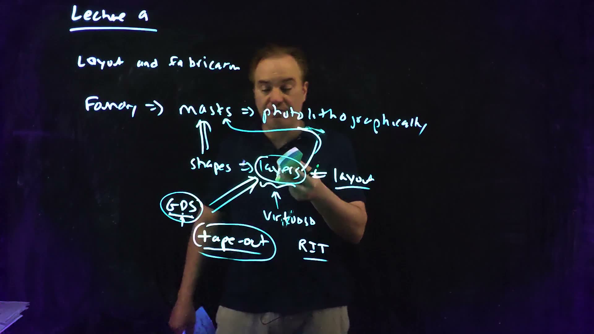
Shapes, layers and masks

The chain runs like this (00:18–01:51) board:

1. The foundry makes a set of masks, which transfer patterns photolithographically onto your wafers, one process step after another.
2. You make the patterns: shapes on a set of predefined layers in a CAD system. In this class that is Cadence Virtuoso (00:45).
3. The foundry combines the layers into the mask definitions. For many layers the mapping is almost one to one; for others, a mask is made from several layers by geometry operations (01:03).
4. The set of shapes on the layers is the layout of your design (01:35).

GDS and tape-out

• The layers go to the foundry in a binary file format called GDS (01:51) board. The lecturer tells its history: it began as the layout format of General Electric’s CAD group in the 1980s, and the name stuck (02:16).
• Sending it is tape-out board. The GDS was once written to a magnetic tape and mailed, so the tape “went out” (03:43). Today the file goes by FTP, but the name remains. At IBM it was a RIT, release interface tape (04:12) board.

The class’s technology

Layer names and definitions differ between nodes and foundries (GlobalFoundries, TSMC, UMC, Samsung), but they are very similar for similar nodes (04:28). The lecture uses the layers of the class’s technology: an old IBM 90 nm process, now run by GlobalFoundries (05:00).

Check yourself What is a layout, and what does the foundry receive at tape-out?

A layout is the design drawn as shapes on the technology’s predefined layers in the CAD system. At tape-out the foundry receives those layers as a GDS file and turns them into masks, one-to-one for most layers and by geometry operations for some.

2. The front-end layers

The idea. Five front-end layers make every transistor and tie: RX opens the silicon, NW makes the well, PC is the poly, BP chooses p+ over n+, and CA contacts the diffusion. What a spot of silicon becomes follows from which of them cover it.

Lecture09 @ 11:12The front-end (FEOL) layers: RX, NW, PC, BP (with reverse toning) and CA.

Front end and back end of the line

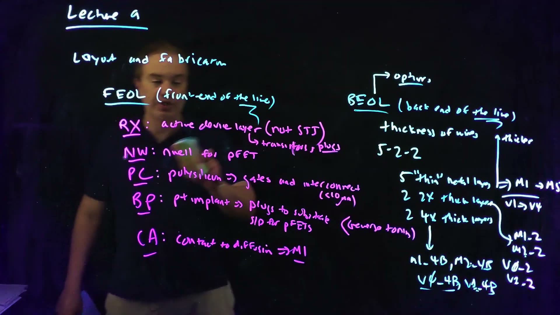
The layers fall into two camps (05:26) board:

• FEOL, front end of the line: the process steps that come first, the layers that make the transistors;
• BEOL, back end of the line: the steps that come last, the layers that make the wires connecting them.

“The line” is the semiconductor production line (06:00). When people talk about “the back end of my process” they mean its wires (06:17).

The five FEOL layers

The two-letter names come from IBM’s old internal layout format, GL1 (07:03). You will see them in Virtuoso (07:29):

Layer	What it is (board)	What it makes
RX	the active device layer: everything that is not STI (07:59)	transistors, and the plugs (substrate and n-well ties) (08:25)
NW	the n well (08:42)	the body for the PFETs
PC	polysilicon (08:57)	gates, and short interconnect: keep poly runs under about 10 µm, since poly is several orders of magnitude more resistive than metal (09:03)
BP	the p+ implant (09:47)	the substrate plugs, and the PFETs’ sources and drains
CA	the contact to diffusion (11:13)	the connection from diffusion up to M1, the first BEOL layer

Two rules decide what you have drawn board:

• PC over RX is a transistor; PC over STI is interconnect (09:37).
• Reverse toning (10:15): BP is the only implant you draw. All RX covered by BP is p+; all RX not covered by BP is n+. There is no n+ layer to draw; n+ is whatever BP leaves out.

Reading the front-end layersboard

$$\text{PC} \cap \text{RX} = \text{gate}$$$$\text{PC} \cap \text{STI} = \text{poly wire}$$$$\text{RX} \cap \text{BP} = p^+, \qquad \text{RX} \setminus \text{BP} = n^+$$

Holds when: the lecture's IBM 90 nm layers on a p substrate; the four RX cases in the table below are added, from the board's rules and Chapter 5's wells

Device or tie? added Add the well and every piece of RX has one meaning:

RX is…	outside NW (p substrate)	inside NW (n well)
not under BP: n+	NFET source or drain	n-well plug (tie), to $V_{DD}$
under BP: p+	substrate plug (tie), to ground	PFET source or drain

The pattern is simple. A source or drain has the opposite doping to the silicon around it (that makes the pn junction). A plug has the same doping as the body it contacts, so it is an ohmic contact into that body. That is why the lecture puts BP “over a PFET” and “over a plug to the substrate” (48:51), and leaves the NFET and the n-well plug without it.

Common mistakes.

• Putting BP over the n-well plug “because it’s in the PFET’s well”. That makes p+ in the n well: a PFET-style diffusion, not a contact to the well.
• Forgetting that poly crossing RX always makes a transistor. A poly wire routed across an active area adds a device.
• Long poly wires. Poly is fine for a short jog (the inverter’s gate connection), not for long interconnect.

Check yourself Which layers do you draw for: an NFET; a PFET; a substrate plug; an n-well plug?

NFET: RX, crossed by PC, no BP, outside NW (CA on its source and drain). PFET: RX crossed by PC, under BP, inside NW. Substrate plug: RX under BP, outside NW (p+ into the p substrate). N-well plug: RX without BP, inside NW (n+ into the n well). Each diffusion and plug also gets CA to reach M1.

Check yourself You draw a PFET but forget the BP over it. What does the foundry build?

Its RX becomes n+ (reverse toning), inside the n well. N+ in an n well is not a transistor’s source and drain: it is the same thing as the n-well plug, a contact to the well. There is no PFET; its “drain” contact simply connects to the well, which is tied to V_DD. DRC can’t catch this (every shape may be legal); LVS will, because the layout no longer has the PFET (Section 6).

3. The back-end layers: the metal stack

The idea. Above the transistors sit layers of metal joined by vias. Wires get thicker going up the stack, so the top layers carry power, clocks and long buses; the thin layers below do local wiring.

Lecture09 @ 16:08The 5-2-2 back end: five thin layers M1–M5, two 2X layers M1_2 and M2_2, two 4X layers M1_4B and M2_4B, with their vias.

Back-end options

A technology usually offers several back-end options for the same transistors (11:37) board. They differ mainly in the thickness of the wires. Going up the stack, the wires get thicker (11:59):

• higher, thicker wires have lower resistance (and, the lecturer says, “actually higher capacitance”; 12:22). That is a good trade where resistance matters most: power grids, clock distribution and long buses (12:40);
• lower, thinner wires have higher resistance but lower capacitance, and do most of the local interconnect (12:55).

added Why thickness lowers resistance: a wire of resistivity $\rho$ρ, length $\ell$ℓ, width $w$ and thickness $t$ has $R = \rho\ell/(wt)$ρℓ/(wt). A 4x-thick wire of the same width has a quarter of the resistance per unit length.

The class’s 5-2-2 back end

The class’s option is called 5-2-2 (13:22) board: five thin metal layers, two 2x thick layers (twice the thickness of the thin ones), and two 4x thick layers (13:25–13:47). The names, top of the stack first, with the via below each (14:05–15:17):

Metal	Thickness	Via below it	The via joins
M2_4B	4x	V1_4B	M1_4B and M2_4B
M1_4B	4x	V0_4B	M2_2 and M1_4B
M2_2	2x	V1_2	M1_2 and M2_2
M1_2	2x	V0_2	M5 and M1_2
M5	thin	V4	M4 and M5
M4	thin	V3	M3 and M4
M3	thin	V2	M2 and M3
M2	thin	V1	M1 and M2
M1	thin	CA	diffusion (or poly) and M1

Every mask derives from these FEOL and BEOL layers (15:32).

Check yourself How many metal layers does a 5-2-2 back end have? Which via joins M5 to the first thick layer, and what would you use the M2_4B layer for?

Nine: M1–M5, M1_2, M2_2, M1_4B, M2_4B. V0_2 joins M5 to M1_2. M2_4B is a 4x-thick layer at the top, lowest resistance: power and clock distribution and long buses (12:40).

4. The layers in cross-section

The idea. Seen from the side, each layer you draw marks where one feature of the device goes. Seen from the top (which is what you draw), the same layers are rectangles.

Lecture09 @ 18:25The cross-section: which layer (RX, BP, PC, CA, NW) defines each region.

The front end, sideways

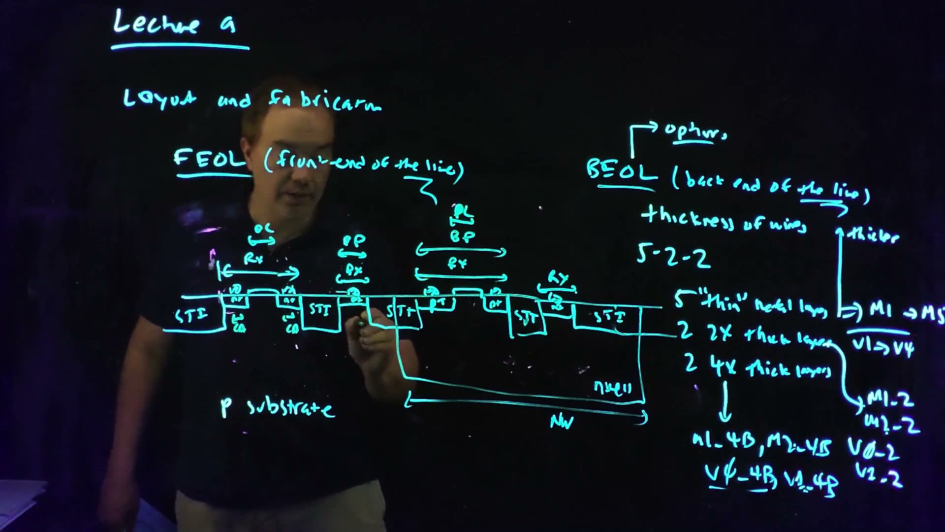
The lecturer draws, left to right on a p substrate (16:30–17:27) board: STI; an NFET (n+, gate, n+); STI; a p+ plug; STI; then, inside the n well, a PFET (p+, gate, p+); STI; an n+ plug; STI. Every diffusion gets a contact. Then he names the layer behind each feature (17:39–18:36) board:

• RX over the four openings in the STI: the NFET, the p+ plug, the PFET and the n+ plug;
• NW over the well;
• BP over the p+ plug and over the PFET, and nowhere else;
• PC over the two gates;
• CA over each of the six contacts.

Check it against Section 2’s table: the n+ plug is RX without BP inside NW; the p+ plug is RX with BP outside NW.

The back end, sideways

Lecture09 @ 24:16The back end in cross-section (CA, M1, V1, M2 in ILD, planarized), and CMP with its two consequences: metal fill and antenna rules.

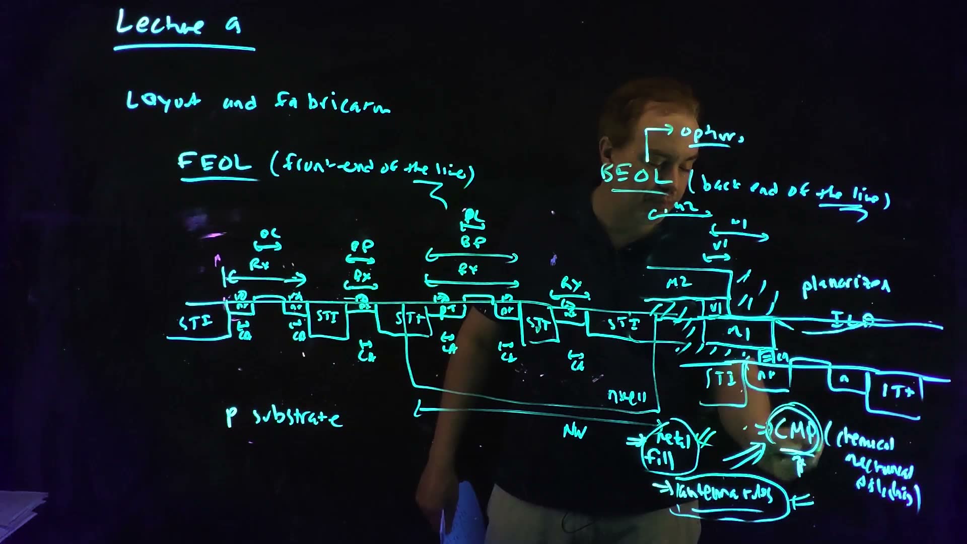
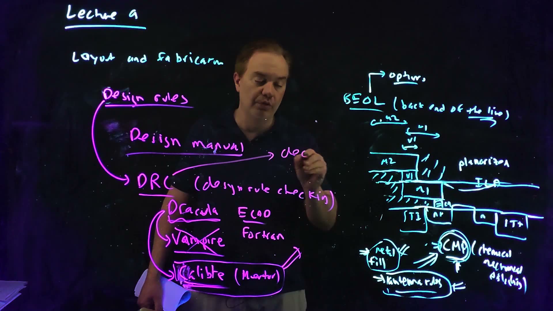
Up from a transistor’s diffusion (19:26) board: CA to M1, then V1 to M2, and so on up the stack. Between the metals is dielectric, the ILD (interlayer dielectric), generally a low-κ material (20:06). The metal layers are planarized: each one is perfectly flat, with no steps over the wires below (20:23).

Check yourself In the 18:25 cross-section, which layers would you draw to make the plug at the right end, inside the n well? Which layer does it not get, and why?

RX (an opening in the STI), NW (it is inside the well) and CA (its contact), with M1 to V_DD. It gets no BP: without BP its RX is n+, the same doping as the n well, so it is an ohmic contact to the well. With BP it would be p+ in the n well, a junction instead of a tie.

5. Planarization: CMP, metal fill and antenna rules

The idea. Polishing each layer flat is what makes tall metal stacks possible, but it imposes two kinds of rule on the layout: a minimum density of metal on each layer, and limits on how metal connects to gates.

Chemical mechanical polishing

After each deposition the fab puts the wafer through CMP, chemical mechanical polishing (20:53) board. It works “like a glorified Brillo pad”: physical and chemical action sand the surface until it is absolutely flat (21:34). Planarizing between layers is what makes very tall stacks possible, 16, 17, 18 levels of metal (21:52). But CMP creates two problems for layout, both in the back end (22:00) board.

Metal fill

Metal and dielectric polish at very different rates. Where a layer has too little metal, CMP can over-etch the dielectric, a problem called dishing (22:29–23:00). So every metal layer must have at least a certain density of metal shapes. If your design doesn’t, you must add dummy metal to bring the density up: metal fill board (23:00).

Antenna rules

Polishing is like walking across a carpet in winter and touching a doorknob: it builds up static charge (23:28). If a piece of metal connected to a gate collects that charge and has no way to discharge it, the charge can blow up the gate (23:50). The antenna rules board are the design rules that prevent this (24:04).

Check yourself A block of logic leaves most of the M4 layer empty over a large area. Why does the foundry care, and what do you do?

CMP needs a minimum metal density on every layer; with too little metal the polish over-etches the dielectric (dishing). You add dummy metal (metal fill) in the empty area until the layer meets the density rule.

Check yourself Why are antenna rules a consequence of CMP, and what do they protect?

Mechanical polishing charges the wafer like static electricity. Metal connected to a transistor’s gate can collect that charge, and if it has nowhere to discharge, the voltage across the thin gate oxide can destroy the gate. The antenna rules limit such connections so the gates survive manufacturing.

6. Design rules and the tools that check them

The idea. The foundry promises that a layout which obeys its design rules will yield. A design-rule checker (DRC) enforces the rules; the same tools also compare the layout with the schematic (LVS) and extract its parasitics.

Lecture09 @ 30:03Design rules, the design manual, DRC and the rule 'deck'; Dracula, Vampire (crossed out) and Calibre.

The design manual

Layout must follow design rules (25:10) board. They are written in the design manual, “a compact between the foundry and the designers” (25:20) board: a PDF in the doc directory of the technology install on the class machines. Rules are things like the minimum width of a shape and the spacing between shapes. The deal: follow every rule and the foundry guarantees your chip will yield, that it can be built and will work; break one and “all bets are off” (25:50–26:30).

DRC

The rules are checked by a DRC tool, design rule checking (26:30) board. The lecturer’s history in two sentences: the first, Dracula (late 1970s, ECAD, written in Fortran), dominated until about 2000; Cadence’s replacement, Vampire, failed, and Mentor’s Calibre took over. Calibre is the tool used in the class (26:45–29:45) board.

• The rules file is still called a deck (29:45) board: in Dracula’s day the rules were a deck of punch cards.
• A layout that runs through the checker with no errors is DRC clean (30:49) board.

LVS and extraction

The checking tools do two more jobs (31:30–32:37):

• LVS, layout versus schematic board: it compares your circuit schematic with the layout and verifies that they match. A layout that passes is LVS clean.
• Extraction board: it extracts the parasitics of the interconnect (resistance, capacitance, sometimes inductance) and builds an equivalent circuit, so you can simulate from the extracted layout.

Calibre does all three: DRC, LVS and parasitic extraction (32:37).

Check yourself An inverter layout is DRC clean, but its PFET drain and NFET drain sit on two separate pieces of M1. Does it work? Which check catches it, and what does each of the three checks establish?

It doesn’t: there is no single output node. DRC can’t see it, since every shape may be legal; DRC checks geometry against the rules. LVS catches it: the layout’s netlist has two output nodes where the schematic has one. Extraction then gives the wiring’s R and C so a simulation of the corrected layout includes them. (Fall 2026’s Lecture 8 asks the same question.)

Check yourself Homework 4 asks for a layout that is “DRC-clean, LVS-clean”, and then for a simulation “of the extracted layout”. Say what each phrase requires.

DRC clean: the design-rule checker (Calibre, with the foundry’s deck) reports no violations. LVS clean: the transistors and connections extracted from the layout match the schematic. Simulation of the extracted layout: run extraction, so the netlist includes the parasitic R and C of the wires, and simulate that netlist instead of the schematic. (This is HW4-1, and HW4-2e–f.)

7. Kinds of design rules

The idea. Most rules are either resolution rules (how narrow and how close shapes on one layer can be) or alignment rules (how far apart shapes on two layers must be). The rest are miscellaneous: fill, antenna, electrical checks.

Lecture09 @ 40:06Three kinds of rules: resolution (width, spacing), alignment, miscellaneous (with ERC); required and recommended rules; LVS and extraction.

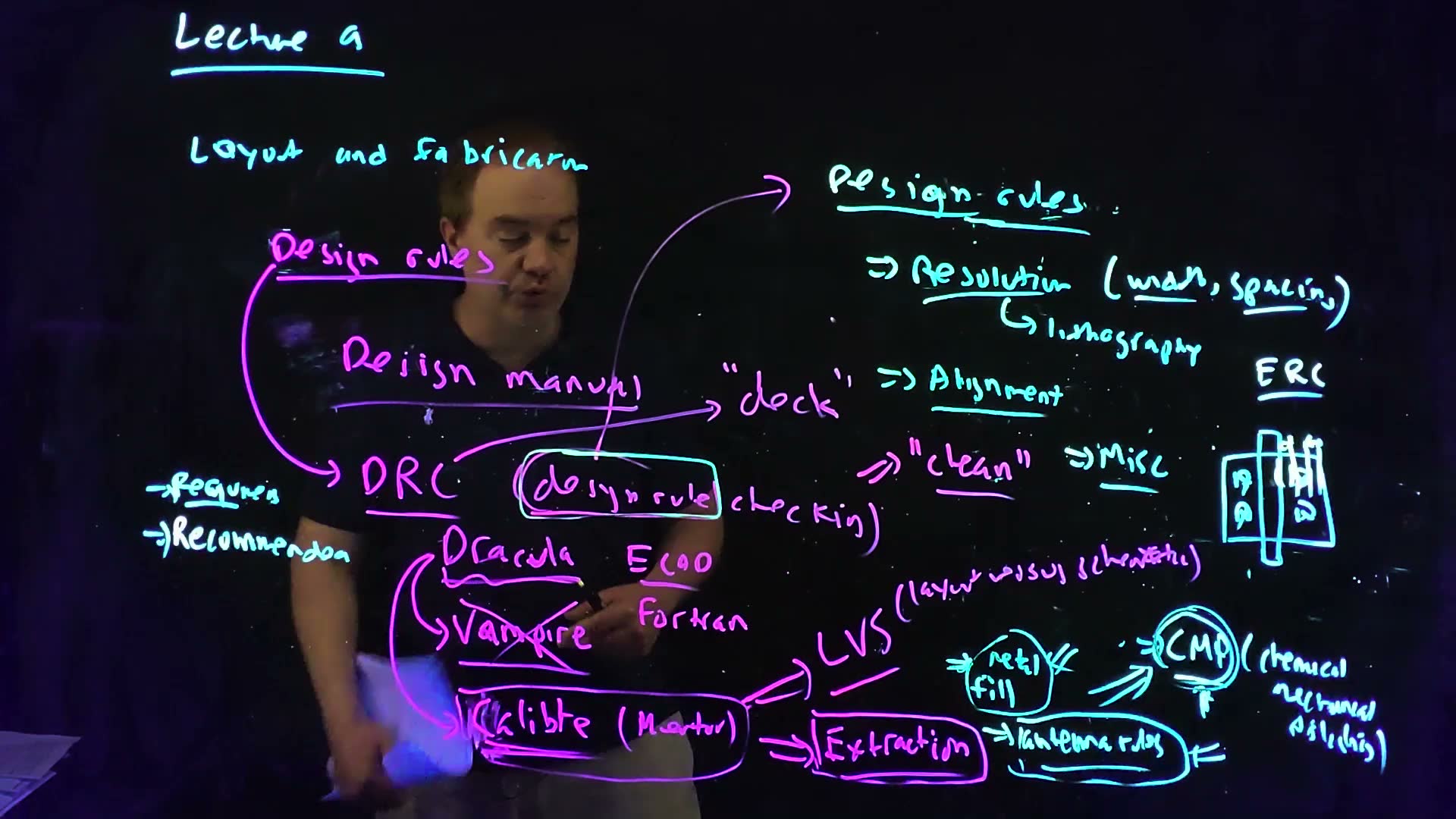
Design manuals grow with every node: a hundred pages once, a thousand or more now (32:58). Modern nodes add strange rules from their lithography tricks; the class’s 90 nm rules are “more normal” and fall into roughly three kinds (34:09) board:

1. Resolution rules (34:20): minimum widths and spacings of shapes on one layer, for example the minimum width of an M1 wire and the minimum space to the next M1 wire. They are set by what the lithography can print.
2. Alignment rules (35:08): minimum spacings between shapes on two different layers, for example how close a contact (CA) may come to the edge of the RX, or to the poly. Each layer has its own mask, aligned to the masks below it with some error; the spacing makes the device work even when the masks are slightly misaligned (36:04).
3. Miscellaneous (36:31): the metal fill requirements, the antenna rules (sometimes a separate deck, but checked by the same tools), and ERC, electrical rule checks such as latch-up rules (36:40).

Contacts: an alignment rule at work

When the lecturer places contacts in the inverter (49:15), three rules decide how many fit: a contact is a fixed-size square, contacts must be a fixed spacing apart, and each must be a minimum distance from the edge of the RX (the alignment rule above). He fits as many as he can.

Contacts in a rowadded

$$W_{min} = a + 2e$$$$n = \left\lfloor \frac{W - 2e + s}{a + s} \right\rfloor$$

Holds when: square contacts of side a, spacing s between contacts, enclosure e from each RX edge, along an RX opening of width W; the three rules are the lecture's (49:15), the count is added

Worked example. added Illustrative rules, invented for this example (not the class’s design manual): contacts $a = 0.12\,\mu\mathrm{m}$ square, spaced $s = 0.14\,\mu\mathrm{m}$0.14μm, at least $e = 0.06\,\mu\mathrm{m}$ inside the RX.

1. The smallest RX that holds one contact: $a + 2e = 0.12 + 0.12 = 0.24\,\mu\mathrm{m}$0.24μm.
2. $n$ contacts in a row take $na + (n - 1)s$1)s, plus $e$ at each end. This must fit in $W$W: $na + (n-1)s + 2e \le W$W, so $n \le (W - 2e + s)/(a + s)$s).
3. An NFET 1 µm wide: $(1 - 0.12 + 0.14)/0.26 = 1.02/0.26 = 3.92$3.92, so 3 contacts. Check: $3(0.12) + 2(0.14) + 0.12 = 0.76\,\mu\mathrm{m} \le 1$1; four would need $1.02\,\mu\mathrm{m}$1.02μm.
4. Its 2 µm PFET: $(2 - 0.12 + 0.14)/0.26 = 7.77$7.77, so 7 contacts.

Required, recommended, and graded

Traditional rules are binary: pass or fail, no grey area (37:36). Yield doesn’t work that way. At IBM, fab engineers would look over DRC-clean layouts and say “if you pulled those two wires further apart … your yield would be better” (38:02). That grew into two sets board: required rules and recommended rules (38:36). The lecturer expects layouts eventually to get a grade, say a score out of 100 with at least 90 needed, so that rules can be traded against each other (38:55–40:01). Today, though, the rules are pass/fail, and that is what you will use (40:01).

Check yourself Sort these rules: (a) M1 at least 0.12 µm wide; (b) CA at least 0.06 µm inside RX; (c) two M2 wires at least 0.14 µm apart; (d) at least 30% of every window covered by M3; (e) CA at least a set distance from a gate's PC.

(a) and (c) are resolution rules: width and spacing on one layer, set by lithography. (b) and (e) are alignment rules: spacing between two layers’ shapes, set by mask-to-mask alignment tolerance (the lecture’s own examples, 35:33). (d) is miscellaneous: a metal-fill (density) rule, from CMP.

8. Layout image

The idea. Give every layer a preferred direction and alternate it going up the stack. Then a route that needs to turn changes layer instead of blocking the layer it is on.

Lecture09 @ 45:16Layout image: a preferred routing direction per layer, alternating up the stack; blockages; routers.

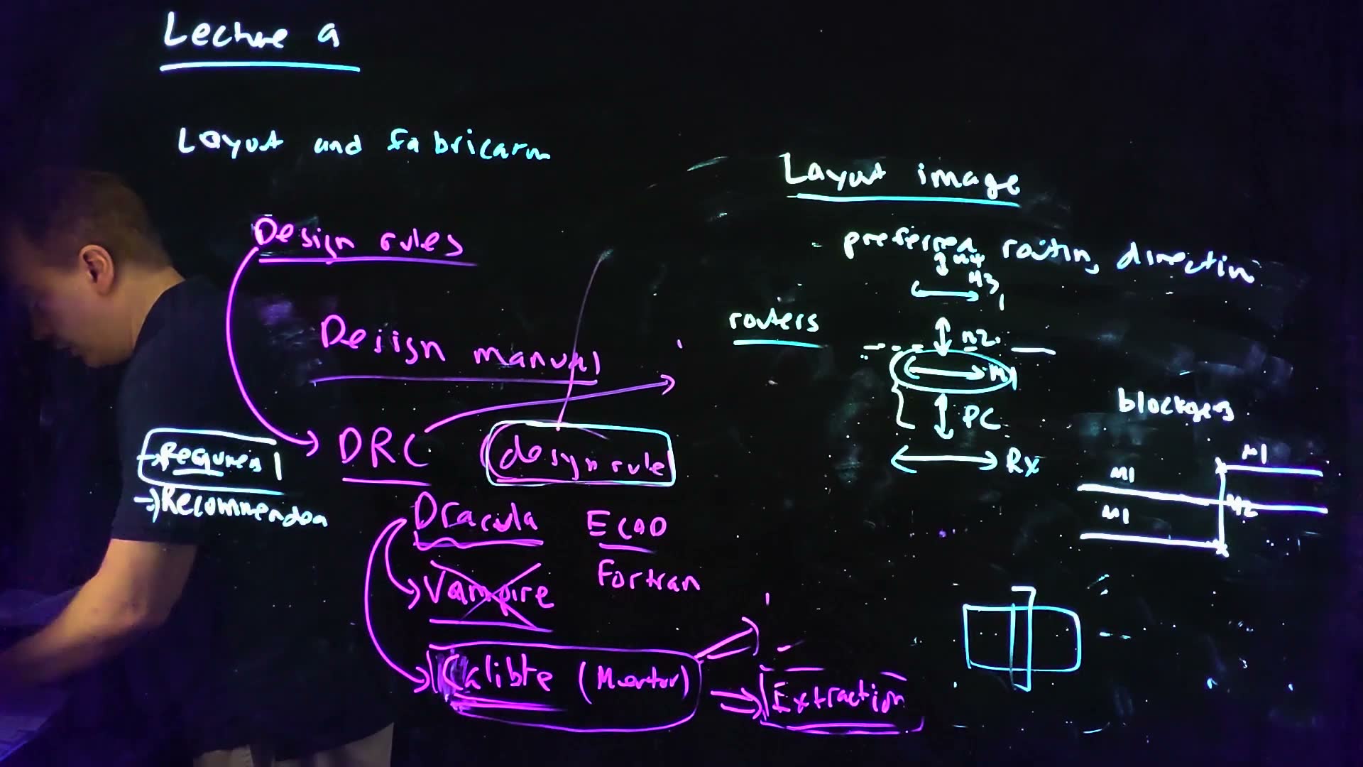
Layout image is a design methodology, not a law, but “a way of organizing your layout that winds up saving you a lot of grief” (40:54). People speak of “following” or “breaking” image (41:09).

• Each layer has a preferred routing direction board (41:36). If the RX runs horizontally, the poly crossing it runs vertically; then M1 horizontally, M2 vertically, M3 horizontally, M4 vertically, alternating all the way up (41:53–42:35).
• Why: blockages board (42:48). Route an M1 wire with a vertical jog in M1, and the next horizontal M1 route is stuck at the jog. Make the jog in M2 instead (via up, jog, via down), and the next M1 route passes straight under it (43:01).
• Automated routers board always follow a preferred direction, because it works so well for routability (43:33).
• In practice, the lowest levels, M1, poly and RX, often break image (44:02). Keeping all poly gates in one direction is good style, and some technologies require it (44:16–44:50). Higher up the stack, follow image closely (44:50).

Check yourself You are routing on M2, whose preferred direction is vertical, and need a short horizontal jog. What does layout image tell you to do, and what goes wrong if you ignore it?

Make the jog on a layer whose preferred direction is horizontal, M1 or M3: via down (or up), jog, and via back. If you jog in M2, the jog crosses the vertical M2 tracks next to it and blocks other vertical routes there.

9. Laying out an inverter

The idea. Draw the two transistors, join their gates in poly, add a plug for each body, put the PFET in a well, mark the p+ regions with BP, contact everything, and wire it in M1.

Lecture09 @ 52:16The finished inverter: vdd! and gnd! rails with their plugs, NW, BP, the poly gate brought out to A, contacts, and M1 to Y.

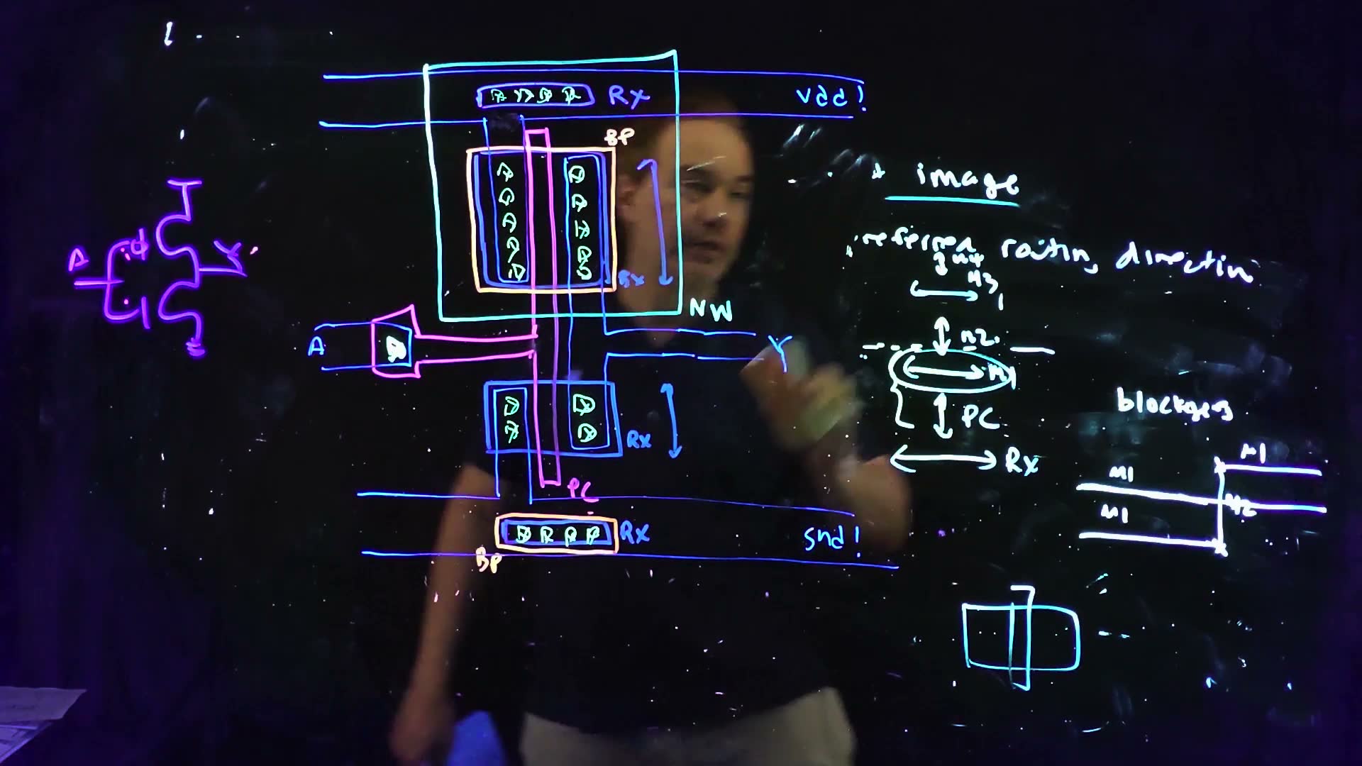
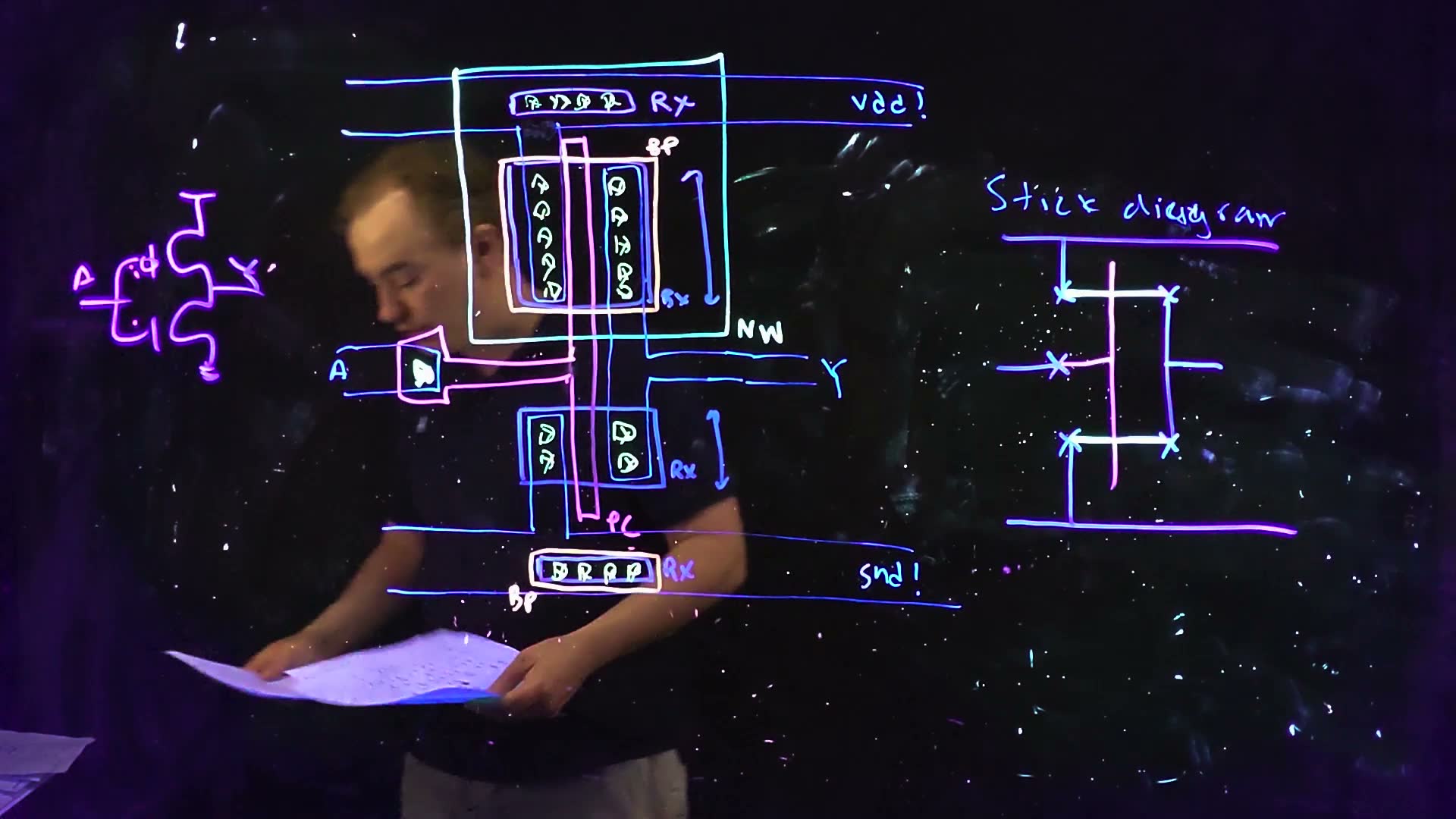
Now the view from the top, which is what you actually draw (45:24). The lecturer lays out an inverter, input A, output Y (46:28) board:

The inverter, in the order drawn (board, 46:38–51:40)

1. RX openings, one for the PFET and one for the NFET. Their height is each transistor’s width (46:38–46:56).
2. PC across both. The two gates are joined in poly: here poly serves as interconnect, which is fine because the jog is short (47:03–47:17).
3. RX for the plugs: a substrate plug and an n-well plug (47:43–48:02).
4. NW around the PFET (48:09), and around its plug.
5. BP over the PFET and over the substrate plug. “And these will be N”: the NFET and the n-well plug get no BP (48:25–48:57).
6. CA: a fixed-size square contact, as many as fit in each diffusion (49:04–49:45; Section 7).
7. The poly brought out to the side and widened, with a CA on it: the connection to the gate (50:03–50:23).
8. M1 rails: vdd! at the top and gnd! at the bottom, Virtuoso’s names for global nets (“VDD bang”) (50:28–50:55). M1 for the output Y and for the input A (51:18).
9. “Oops, missing one thing”: M1 from the PFET’s source up to vdd! and from the NFET’s source down to gnd! (51:25–51:36).

“Here’s my inverter … And it has all my plugs and all my ties” (51:40–52:00). Build it yourself, one step at a time, and probe what each spot of silicon becomes:

◀ BackNext ▶Start overFinished layout

Step 9 of 9 (51:25): "Missing one thing": M1 from the PFET source up to vdd! and the NFET source down to gnd!.

NW (n-well) RX (active) BP (p+ implant) PC (poly) CA (contact) M1 (metal 1)

PFET, left diffusionPFET, under the polyNFET, right diffusiontop plugbottom plugpoly between the gatesinput padempty field

layers here

NW, RX, BP, CA, M1

diffusion here

p+

contact to M1

yes, net vdd!

RX under BP inside NW: p+ in the n-well, a PFET source or drain

Click or tap anywhere on the drawing, or use the spot buttons. The probe reads only the layers drawn so far and shown, so hiding a layer shows what the silicon would become without it: hide BP and probe the PFET's diffusion, or the bottom plug. The drawing follows the board's arrangement (rails at top and bottom, the PFET in its n-well above the NFET, the input brought out to the left); its proportions are not to scale, and it has fewer contacts than the board. The PFET is drawn twice as tall as the NFET, as on the board; no widths were given.

What to notice.

• The PFET’s diffusion and the bottom plug are both under BP, so both are p+; only the well tells them apart. Hide NW and probe the PFET: it reads as a substrate plug.
• Hide BP and probe the PFET’s diffusion: it becomes n+ in the n well, a well plug. That is reverse toning; Section 2’s second check.
• The poly between the two gates is over STI: a wire, not a transistor.

Which net is which. added Reading the finished layout:

Net	What it connects
vdd!	PFET source, n-well plug
gnd!	NFET source, substrate plug
A	both gates (through the poly pad and its contact)
Y	PFET drain and NFET drain

The plugs go to the rails for the reason in Chapter 5: with the substrate at ground and the well at $V_{DD}$VDD​, no source or drain junction can be forward-biased.

The tools help. Virtuoso’s P-cells (parameterized cells) draw a transistor’s layers for you from its width and number of fingers, so you don’t redraw them each time (52:26). The XL version of the layout tool tracks the connectivity from the schematic and guides your wiring (53:25).

Check yourself In the lecture's inverter, why are there two plugs, why does only one of them get BP, and where does each connect?

Each body needs a tie: the p substrate (under the NFET) and the n well (under the PFET). The substrate plug is p+, so it gets BP, and connects to gnd!. The well plug is n+, so it gets no BP, and connects to vdd!. Each plug has the doping of the body it contacts, and the rails keep every junction reverse-biased.

Check yourself The lecturer draws the PFET's RX opening about twice as tall as the NFET's. What is he drawing, and why that ratio?

The height of the RX opening, under the poly, is the transistor’s width (46:56). A 2:1 ratio is the usual 2W/W inverter: the PFET is twice as wide so that, with R_pfet ≈ 2R_nfet, its rising delay matches the NFET’s falling delay (Chapter 7). No widths were given on the board.

10. Stick diagrams

The idea. Before drawing a real layout, sketch it with one line per diffusion, one per poly gate and one per metal wire. The sketch shows where the transistors are, which diffusions they share, and how they connect.

Lecture09 @ 56:58The inverter's stick diagram: diffusion lines, a poly line, metal lines and X contacts.

The lecture’s stick diagram

Laying out in Virtuoso takes work, so you plan first (53:28). A stick diagram is a shorthand for the layout that you can draw very quickly (54:09) board. For the inverter (54:30–55:20):

• a line for each diffusion: one for the N, one for the P;
• a line for the poly gate, crossing both;
• lines for metal: power and ground, the output joining the two diffusions, the input coming in to the poly;
• a mark for each contact (an X on the board).

“That’s why they’re called stick diagrams, because you’re drawing them like sticks” (54:37). The point is planning: you can see at once where you will share diffusions and how many fingers to give each device, before committing to the full layout (55:31). The next lecture plans layouts this way.

Reading a stick diagram

added The midterms turn this around: they give a stick layout and ask for the schematic and the logic function (MT23-4, MT24-4). The rules for reading one come straight from Section 2 and from Chapter 5’s sharing diffusions:

1. Find the rows. The diffusion line nearer $V_{DD}$ (or in the well, or labelled p) is the PFET row; the one nearer ground is the NFET row.
2. Every poly line crossing a diffusion line is one transistor, with that poly’s signal on its gate (PC over RX is a transistor).
3. The pieces of diffusion between poly lines are the nodes. Two transistors next to each other on one line share the piece between them.
4. An X joins a piece to the metal through it. Follow the metal to name the node: $V_{DD}$VDD​, GND, the output, or a wire to another poly.
5. An uncontacted piece joins only its two neighbours: they are in series. Two transistors whose outer ends reach the same pair of nodes are in parallel.
6. Write the pull-up and pull-down networks, then the function.

Worked reading. added Gate 1 in the widget below.

Reading gate 1

1. Two poly lines, A and B, each cross both diffusion lines: four transistors, two PFETs and two NFETs.
2. PFET row, left to right: X to $V_{DD}$VDD​, poly A, X to the output Y, poly B, X to $V_{DD}$VDD​. PFET A runs from $V_{DD}$ to Y, PFET B from Y to $V_{DD}$VDD​: both between $V_{DD}$ and Y, so they are in parallel.
3. NFET row: X to GND, poly A, an uncontacted piece, poly B, X to Y. NFET A runs from GND to the middle piece, NFET B from the middle piece to Y: the middle node goes nowhere else, so they are in series.
4. Parallel PFETs over series NFETs: Y is pulled low only when A and B are both 1. $Y = \overline{AB}$AB, a NAND.

Read the others yourself before you press “Show the function”. Set the inputs and watch which transistors conduct:

Inverter (the lecture’s)Gate 1Gate 2Gate 3 (two stages)

A = 0

p diffusion n diffusion poly metal 1✕ contact

output Y

1

transistors read

2

type	gate	between	now
PFET	A	VDD – Y	on
NFET	A	GND – Y	off

Show the function

Green squares mark transistors that conduct for the inputs set; grey ones are off (an NFET conducts on a 1, a PFET on a 0). "Internal" is a piece of diffusion with no contact: it joins only the two transistors on either side of it. The inverter is the lecture's (board 56:58); gates 1–3 are added for practice, in the same style.

What to notice.

• In gate 2 the NFETs share a contacted piece (to GND) between them, and their outer ends both reach Y: parallel. That is Chapter 5’s “share the sources” pattern.
• In gate 3 the first stage’s output is a metal line ending in an X on the second stage’s poly: one gate driving another, the way the lecture’s input A reaches its poly.
• A piece with no X never appears in the readout as a named net: it is “internal”, shared only by its two neighbours.

Common mistakes.

• Treating a poly line that crosses both rows as one transistor. It is two: a PFET where it crosses the P line and an NFET where it crosses the N line, with the same gate signal.
• Assuming metal crossing a diffusion or a poly line connects to it. Only an X (a contact) connects layers.
• Reading series for parallel. Check where each transistor’s two ends go, not just whether it sits next to another one.

Exam-style practice. added A gate in the style of MT24-4:

p diffusion n diffusion poly metal 1✕ contact

Check yourself Read the stick layout above (A and B enter on the poly from the bottom; ✕ marks a contact). Draw the schematic. What logic function is Z?

First stage (left), PFET row: V_DD, A, an uncontacted piece, B, then a contact to node X: PFETs A and B in series from V_DD to X. NFET row: X, A, GND, B, X: both NFETs run from GND to X, in parallel. So X = NOT(A + B), a NOR. The metal from X ends in a contact on the second stage’s poly. Second stage: one PFET from V_DD to Z and one NFET from GND to Z, both gated by X: an inverter. $Z = \overline{X} = A + B$B, an OR gate. (MT24-4 asks the same for three inputs; the exam kit re-solves it.)

Check yourself Homework 4 asks for a stick diagram of a chain of three inverters (IN → X → Y → OUT) before the layout. Describe it.

Three copies of the lecture’s stick diagram side by side, sharing the V_DD and ground rails: in each, a P line and an N line crossed by one poly line, X contacts at both ends of both lines, the outer ends to the rails, the inner ends joined by a metal line. That metal line (X, then Y) runs to an X on the next inverter’s poly; IN comes in on the first poly and OUT leaves from the last metal line. (This is HW4-1a.)

What comes next

The lecturer stops here (56:02). The next lecture goes back to diffusion sharing: planning it with stick diagrams for bigger gates and moving the plan into layout, the layout-dependent device models that let a schematic know which diffusions are shared, and multi-finger transistors (56:21–56:57). That is Chapter 10.

Formulas to remember

Rule	Meaning
shapes on layers → masks; GDS; tape-out (RIT)	the layout and how it reaches the foundry
FEOL: transistors; BEOL: wires	front and back end of the line
RX active (not STI); NW n well; PC poly; BP p+ implant; CA contact to M1	the five FEOL layers
PC ∩ RX = transistor; PC over STI = wire (keep under about 10 µm)	poly
RX under BP = p+; RX not under BP = n+	reverse toning
n+ outside NW = NFET S/D; p+ in NW = PFET S/D; p+ outside NW = substrate plug (gnd); n+ in NW = well plug ($V_{DD}$VDD​)	device or tie
5-2-2: M1–M5 (V1–V4), M1_2, M2_2 (V0_2, V1_2), M1_4B, M2_4B (V0_4B, V1_4B)	the class’s metal stack; thicker going up
CMP → metal fill (density) and antenna rules	planarization’s two consequences
DRC: geometry vs rules; LVS: layout vs schematic; extraction: wire R, C	the three checks (Calibre)
resolution (width, spacing; one layer), alignment (two layers), misc (fill, antenna, ERC)	kinds of design rule
$n = \lfloor (W - 2e + s)/(a + s) \rfloor$	contacts in a row (added)
alternate preferred directions up the stack	layout image; avoids blockages
poly crossing diffusion = transistor; uncontacted shared piece = series; same two end nodes = parallel	reading a stick diagram (added)

The lecture’s boards

Lecture09 @ 05:03 foundry, masks, layers, layout; GDS, tape-out, RIT

Lecture09 @ 11:12 FEOL layers RX, NW, PC, BP, CA; reverse toning

Lecture09 @ 16:08 BEOL: the 5-2-2 metal stack

Lecture09 @ 18:25 the front end in cross-section

Lecture09 @ 24:16 the back end; CMP, metal fill, antenna rules

Lecture09 @ 30:03 design manual, DRC, the deck; Dracula to Calibre

Lecture09 @ 40:06 resolution, alignment, misc; LVS, extraction

Lecture09 @ 45:16 layout image; blockages

Lecture09 @ 52:16 the inverter layout

Lecture09 @ 56:58 the inverter stick diagram