H3. Homework 3: delay calibration, crowbar energy and path sizing

Homework 3 is where the course’s delay model gets its numbers. Problem 1 measures the gate capacitance $C_g$ and the “resistances” $R_{nfet}$ and $R_{pfet}$ that every later delay estimate uses, plus the drain capacitance $C_d$Cd​. Problem 2 measures the energy an inverter draws, and how much of it the crowbar current wastes. Problem 3 sizes a three-gate path by logical effort and picks the number of stages. Problems 1 and 2 are circuit simulations; Problem 3 is a hand calculation, the same method as the path-sizing questions on every midterm.

How to read this page.

• The sources hold only the solution to Homework 3, not the handout. Each question below is reconstructed from the key’s own wording and figures, and says so.
• There is no simulator here, and this page invents no simulation numbers. For Problems 1 and 2 it teaches what the bench measures, which node to watch and which formula turns the reading into a parameter. The key’s simulated values appear as readings from the key’s plot (or its simulation), and the arithmetic on them is redone and checked.
• Problem 3 is re-solved from scratch, and every number is checked.
• The simulation questions open with a How to approach section: how to recognize them, the moves in order, why the formulas apply, and the traps. Then every part is worked the same way: what it asks, the idea behind the method, the solution in steps (each step gives its reason first), a check on the result, the answer, and one thing to remember. Try each part on your own first; open the Hint if you are stuck. The answer key’s verdict is the folded note on the key at the end of the part.

Before you start. The methods are in these sections:

• the two benches and their formulas (Chapter 7 §2, §3), and the FO1 delay $\tau_{inv} = 3R_nC_g$ (Chapter 7 §7);
• overlap and junction capacitance, and $\eta = C_g/C_d$ (Chapter 5 §4, §5, §11);
• switching energy and crowbar current (Chapter 6 §6, §7), and the saturated-ramp transient (§9);
• gains from the normalized inverter, equal-gain sizing and the number of stages (Chapter 8 §1, §3, §4, §6, §7).

How to approach a simulation-bench question

Recognize it by the picture, a Cadence schematic built with the technology’s models, and by the phrases “find by simulation”, “using the method discussed in class” and a unit to report (“in fF/µm”, “in kΩ·µm”). The question gives you no numbers to compute from. You build a circuit, read a delay or a current off the simulator, and turn the reading into a parameter. Problems 1 and 2 are this family; so are Homework 2’s I–V benches (H2 §1) and the timing of an extracted layout in Homework 4. The homework carries no exam points. On the midterms the benches’ results come back as given numbers (“$C_g = 2$Cg​= fF/µm, $R_n = 4\,\mathrm{k\Omega\cdot\mu m}$4kΩ⋅μm”) and their reasoning as short answers.

The moves, in order.

1. Say what the bench holds fixed and what it sweeps. Bench 1 holds two identical inverters and sweeps a capacitor; bench 2 holds three inverters and reads two delays; Problem 2 holds the inverter and its load and changes the input ramp.
2. Say what cancels. Two identical stages fed the same waveform carry the same drain capacitance, so a comparison between them removes it. Where a delay is divided by a gate load instead, the drain areas are zeroed (AS = AD = PS = PD = 0), so that nothing else is in the load.
3. Name the node to watch, and the edge. The outputs whose delays you compare, timed from their common input; or the supply current, which flows through the PFET, for an energy.
4. Write the one formula from reading to parameter. $C_g = C_L/(\text{the gate width it replaces})$CL​/(the gate width it replaces); $R = t_p \times W/C_L$W/CL​; $E = V_{DD}\int i_{DD}\,dt$VDD​∫iDD​dt.
5. Check against a number you know. In the course’s model the fan-out-of-four delay is $\mathrm{FO4} = 4\tau_{inv} = 12R_nC_g$ for a 2W/W inverter added (Chapter 7 §7), so your $R_n$ and $C_g$ must give back the FO4 you measured. With the key’s FO4 and its $C_g$Cg​, that fixes what $R_n$ must be (HW3-1b works it out). A result off by a factor of 2 has the wrong load or the wrong edge.

Why these formulas.

• Equal delays mean equal loads. A stage’s delay is set by its strength and its load. Two identical inverters driven by the same waveform have the same strength, so if their delays match, their loads match, whatever the devices do in detail. That is how a plain capacitor can measure a gate (Chapter 7 §3).
• Delay $= (R/W)\,C$(R/W)C. The course models the conducting transistor as a resistance $R/W$R/W, with $R$ in kΩ·µm, that charges or discharges the load $C$C; 1 kΩ × 1 fF = 1 ps. It holds for minimum-length devices and gate loading only, drain capacitance ignored (Chapter 7 §2). Turned around, $R = t_p\,W/C_L$tp​W/CL​.
• $E = V_{DD}\int i_{DD}\,dt$VDD​∫iDD​dt. Power from a fixed supply is $V_{DD}\,i_{DD}$VDD​iDD​, so the energy of an edge is $V_{DD}$ times the charge the supply delivers (Chapter 6 §6). Charging $C_L$ to $V_{DD}$ delivers the charge $C_LV_{DD}$ whatever the waveform, so a rising output draws at least $C_LV_{DD}^2$CL​VDD2​. Crowbar current, which flows straight from $V_{DD}$ to ground while both devices conduct, adds to it (Chapter 6 §7).

Decisions to make on the way.

• Which edge. A rising output is the PFET’s job: $t_{pLH}$ gives $R_{pfet}$Rpfet​, and only a rising output draws the load’s charge from the supply. A falling output is the NFET’s: $t_{pHL}$ gives $R_{nfet}$Rnfet​.
• Which load. The receiving inverter’s whole gate: both of its devices, times its multiplier. That is $8(16 + 8)\,\mu$m in bench 1 and $16(16 + 8)\,\mu$m in bench 2. The width you multiply by is the measured device’s own: $4(8\,\mu\mathrm{m})$ for bench 2’s NFET.

Traps. The wrong load: HW3-1b’s key divides by bench 1’s 168 fF and gets resistances twice too large. Per edge against per cycle: a cycle costs $C_LV_{DD}^2$ plus both edges’ crowbar, not twice one edge. Calling the whole excess crowbar: the driver also charges its own drains. An $\eta = C_g/C_d$ outside Lecture 5’s 1.5–2: say so rather than pass over it. Units: $R$ is in kΩ·µm, not kΩ.

1. HW3-1: calibrating the delay model

The task (HW3-1, p1–3, reconstructed from the key). With the technology’s simulation models (the figures show 60 nm devices and a 1 V supply), find (a) the gate capacitance $C_g$ in fF/µm, (b) $R_{nfet}$ and $R_{pfet}$ in kΩ·µm, and (c) the drain capacitance $C_d$ of each device type on each transition, “using the method discussed in class”. That method is Lecture 7’s two fan-out-of-four benches (Chapter 7 §3).

These three numbers are what the exams hand you: “$C_g = 2$Cg​= fF/µm, $R_n = 4\,\mathrm{k\Omega\cdot\mu m}$4kΩ⋅μm” in Problem 3 below, and in every midterm’s delay question. HW3-1 is where such numbers come from.

HW3-1a: gate capacitance (p1)

HW3-1a, p1 (the key’s bench). Top row: 16/8 → 2(16/8) → 8(16/8). Bottom: a second 2(16/8) drives the capacitor C0.

Hint

The two 2(16/8) inverters are identical and share one input. What does it tell you when their delays come out equal?

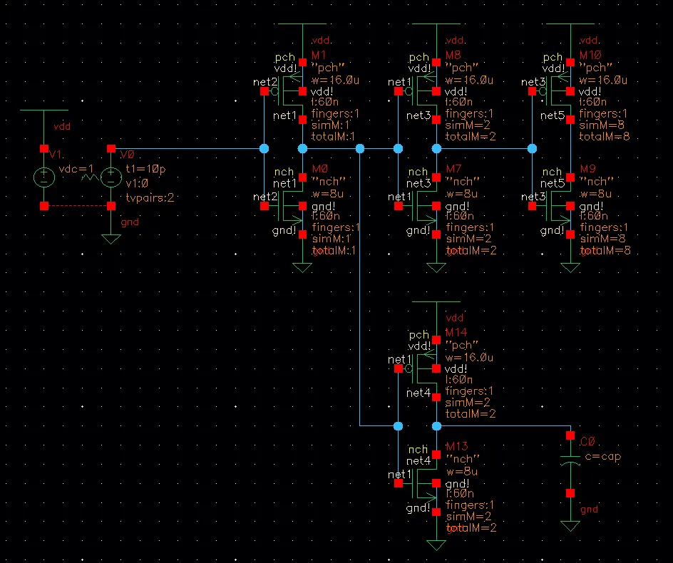
What it asks. The gate capacitance per micron of gate width, $C_g$ in fF/µm, found by simulation “using the method discussed in class”. The simulator won’t show you a gate’s capacitance directly, but it shows delays. The method turns a delay comparison into a capacitance.

The idea. This is Lecture 7’s bench 1 (Chapter 7, Bench 1). The 16/8 inverter drives two 2(16/8) inverters, a fan-out of four. The two are identical and share one input, so they are equally strong. One drives an 8(16/8) inverter, a gate load of unknown capacitance; the other drives a plain capacitor $C_L$CL​, which the bench sweeps. In the delay model each takes $(R/W)\,C_{load}$ with the same $R/W$R/W, so their delays are equal exactly when their loads are: when $C_L$ equals the 8(16/8) inverter’s input. Their own drain capacitance is the same on both, so it adds equally to both delays and cancels (Chapter 7, “Zero the drain capacitance”). The nodes to watch are the two 2(16/8) outputs (net3 and net4), timed from their common input net1. At the match, divide $C_L$ by the gate width it stands in for:

$$C_g = \frac{C_L}{8\,(16 + 8)\,\mu\mathrm{m}}$$

The bench’s other two details follow the lecture. The first inverter is wide (“$W >$W> a few microns”) so that the drawn-width correction $\Delta W$ is negligible. The input ramp is about twice the FO4 delay (the key measured FO4 ≈ 14.3 ps), and the first inverter turns it into a realistic FO4 edge.

HW3-1a

1. Read the match. The sweep stops where the two delays are equal. The key’s reading: $C_L \approx 168$ fF, with both delays near 15.8 ps (readings from the key’s simulation).
2. Count the gate the capacitor stands in for. An inverter’s input is wired to both of its gates, and the multiplier 8 puts eight copies in parallel: $8 \times (16 + 8) = 192\,\mu\mathrm{m}$ of gate.
3. Divide. 168 fF is the capacitance of 192 µm of gate, so $C_g = \dfrac{168\,\mathrm{fF}}{192\,\mu\mathrm{m}} = 0.875\,\mathrm{fF/\mu m}$0.875fF/μm.

Check. The matched stage is itself a fan-out-of-four stage: a 2(16/8) inverter driving an 8(16/8), four times its size. So its delay at the match should be close to the FO4 delay the key measured on its own, 14.3 ps. It is 15.8 ps, within about 10% ($15.8/14.3 = 1.10$15.8/14.3=1.10).

Answer: $C_g \approx 0.875$ fF/µm.

Remember. Identical drivers with equal delays have equal loads. To measure a capacitance you can’t see, match it with one you can, then divide by the gate width it replaces.

The answer key agrees

HW3-1b: resistance (p2)

HW3-1b, p2 (the key’s bench): 16/8 → 4(16/8) → 16(16/8). The middle inverter is the one measured.

Hint

Which inverter’s delay is measured, and what exactly does it drive?

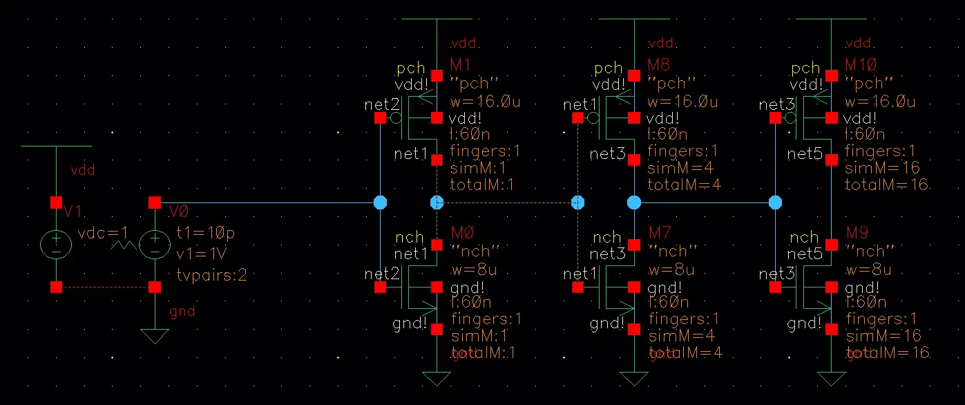
What it asks. The “resistance” of each device type, $R_{nfet}$ and $R_{pfet}$Rpfet​, in kΩ·µm: the number that, divided by a device’s width, gives the resistance it acts as. Again the simulator gives only delays. The unit decides the last step: kΩ·µm is a resistance multiplied by the measured device’s width.

The idea. This is Lecture 7’s bench 2 (Chapter 7, Bench 2). It holds three inverters in a row, 16/8, 4(16/8) and 16(16/8), each at fan-out of four. The first cleans up the ramp, the last is a known gate load, and the middle one, 4(16/8), is measured. Nothing is swept: you read two delays at the middle inverter’s output. Its falling delay $t_{pHL}$ is the NFET’s job (the NFET discharges the output), and its rising delay $t_{pLH}$ is the PFET’s. In the delay model a device of width $W$ drives a load $C$ in $(R/W)\,C$(R/W)C, with 1 kΩ × 1 fF = 1 ps (Chapter 7 §2). That holds for gate loading only, so the bench sets AS = AD = PS = PD = 0 and the middle inverter’s own drain capacitance is gone. Turned around:

$$R_{nfet} = \frac{t_{pHL}}{C_L}\times 4(8\,\mu\mathrm{m})$$ $$R_{pfet} = \frac{t_{pLH}}{C_L}\times 4(16\,\mu\mathrm{m})$$ $$C_L = C_g \times 16(16+8)\,\mu\mathrm{m}$$

The tempting slip is the load. Bench 1’s capacitor stood in for an 8(16/8) inverter; here the load is a 16(16/8), twice as much gate. The key writes the formula as $R = \dfrac{t_p}{C_g}\times W$W: read $C_g$ there as the load capacitance $C_L$CL​, not the per-micron 0.875.

HW3-1b

1. Find the load. The middle inverter drives the 16(16/8) inverter’s input, both gates of sixteen copies: $C_L = 0.875 \times 16 \times 24 = 336\,\mathrm{fF}$336fF.
2. Work back to the delays. The key prints no delays, only its results, $R_n = 2.78$ and $R_p = 5.69$ (“kΩ”; the unit is kΩ·µm). So turn the formula around to see what delays they imply: $t_{pHL} = \dfrac{2.78 \times 336}{32} = 29.2\,\mathrm{ps}$ and $t_{pLH} = \dfrac{5.69 \times 336}{64} = 29.9\,\mathrm{ps}$29.9ps.
3. Compare with the key’s own measurement. The middle inverter drives four times its own size, so its delay is an FO4 delay. The key says these delays are “very similar to our FO4 delay”, which it measured at 14.3 ps. The implied 29 ps is about twice that.
4. Run the same test in the model. The model’s FO4 is $4\tau_{inv} = 12R_nC_g$ added (Chapter 7 §3). With the key’s numbers that is $12 \times 2.78 \times 0.875 = 29.2$ ps, again twice the measured FO4.
5. Redo it with delays near the measured FO4. Since the middle inverter is an FO4 stage, its delays must be near 14.3–15.8 ps. The formula then gives $R_n = 1.36$–$1.50\,\mathrm{k\Omega\cdot\mu m}$ and $R_p = 2.72$–$3.01\,\mathrm{k\Omega\cdot\mu m}$3.01kΩ⋅μm.
6. Look at the ratio. Both resistances are divided by the same load, so the ratio doesn’t depend on the slip: $R_p/R_n = 5.69/2.78 = 2.05$2.05, the expected “PFET has half the drive”.

Check. Bench 1 gives a second route. Its matched stage, a 2(16/8) inverter whose NFET is 16 µm wide, drives 168 fF: the same FO4 stage at half the size, so the model gives it the same delay, $(R_n/16) \times 168 = (R_n/32) \times 336$336. Its measured 15.8 ps therefore means $R_n = 15.8 \times 16/168 = 1.50\,\mathrm{k\Omega\cdot\mu m}$1.50kΩ⋅μm, inside the range of step 5. The key’s 2.78 would need 29.2 ps there.

Answer: $R_n \approx 1.4\,\mathrm{k\Omega\cdot\mu m}$ and $R_p \approx 2.8\,\mathrm{k\Omega\cdot\mu m}$2.8kΩ⋅μm, from delays near the key’s FO4; $R_p \approx 2R_n$2Rn​. Then $\tau_{inv} = 3R_nC_g \approx 3.65$ ps and FO4 $= 4\tau_{inv} \approx 14.6$ ps, which matches the key’s 14.3 ps.

Remember. Bench 2: $R$ = the delay × the measured device’s width ÷ the receiving inverter’s whole gate load. Then test the result: $12R_nC_g$ must give back the FO4 delay you measured.

The answer key differs

It gives $R_n = 2.78$ kΩ and $R_p = 5.69$ kΩ. Those values need middle-inverter delays of 29.2 and 29.9 ps, twice the 14.3 ps FO4 delay the key says they resemble. They follow exactly if the delays were 14.6 and 14.9 ps and the key divided by 168 fF (bench 1’s capacitor, an 8(16/8) load) instead of the 336 fF of the 16(16/8) inverter in its own figure. With 336 fF the same delays give $R_n = 1.39$ and $R_p = 2.85\,\mathrm{k\Omega\cdot\mu m}$2.85kΩ⋅μm. The key prints no delays, so this is a reconstruction; but either way its resistances contradict its own FO4. The unit is kΩ·µm, not kΩ.

HW3-1c: drain capacitance (p3)

HW3-1c, p3 (the key’s bench for a PFET). The capacitor of 1a is replaced by the drain of M16, an off PFET: w = 16.6 µm, multiplier 16 (zoomed in on the source figure).

Hint

If you hung a transistor on the lower 2(16/8) inverter in place of the capacitor, what would it add to the node if it conducted?

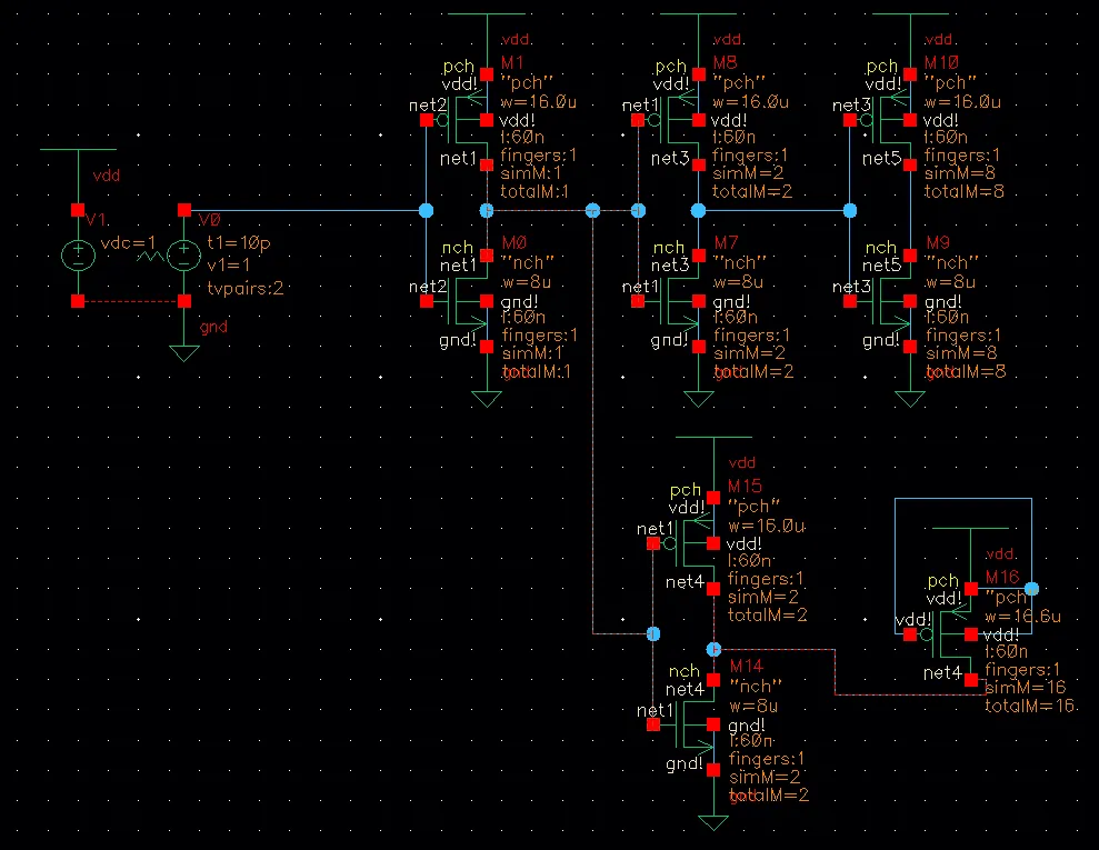
What it asks. The drain capacitance per micron of width, $C_d$Cd​, for each device type and each output transition: four numbers. The words “on each transition” decide that you measure each case separately, because a junction’s capacitance depends on the voltage across it.

The idea. Bench 1 again, with the capacitor replaced by the drain of a transistor that is off: a PFET with its gate tied to $V_{DD}$VDD​, or an NFET with its gate grounded. It must be off. A conducting device would carry current and add its gate capacitance to the node; an off one forms no channel, so the node sees only its drain’s junction capacitance (Chapter 5 §5) and its overlap to the gate (§4). The two 2(16/8) drivers are still identical, so their own drains still cancel, and the nodes to watch are still their outputs, net3 and net4, timed from net1 (1a). Sweep the off device’s width until the two delays match again. Then its drain loads the node as much as the 8(16/8) gate does:

$$C_d\,W_{match} = C_g \times 8(16+8)\,\mu\mathrm{m} = 168\,\mathrm{fF}$$ $$C_d = \frac{168\,\mathrm{fF}}{W_{match}}$$

This bench is not in Lecture 7, whose model zeroes $C_d$Cd​. It is Lecture 5’s drain capacitance measured with Lecture 7’s matching idea.

HW3-1c

1. Read the matched width off the figure. The key’s figure shows the matched PFET for one case: $16 \times 16.6 = 265.6\,\mu\mathrm{m}$ of drain. So $C_d = 168/265.6 = 0.633\,\mathrm{fF/\mu m}$0.633fF/μm: the key’s P,HL value.
2. Turn the other readings around. The key’s four values are readings from its simulation. Since $W_{match} = 168/C_d$168/Cd​, each value fixes a matched width; the table gives them, with $\eta = C_g/C_d$ for $C_g = 0.875$ fF/µm, the ratio Lecture 5 uses.
3. Say why the edges differ. Junction capacitance depends on the voltage across the junction (Chapter 5 §5), and a delay match weighs the part of the swing near the 50% crossing. A falling and a rising output sweep the junction through different voltages, so they see different capacitances.

Device, output edge	$C_d$ (fF/µm)	$W_{match}$ (µm)	$\eta = C_g/C_d$
PFET, falling (HL)	0.63	267	1.39
PFET, rising (LH)	0.50	336	1.75
NFET, falling (HL)	0.66	255	1.33
NFET, rising (LH)	0.73	230	1.20

Check. Every $C_d$ in the table is below $C_g = 0.875$ fF/µm, so every $\eta$ is above 1, as an off drain should give: it offers only a junction and an overlap, while a gate has its whole area over a thin oxide. The PFET’s rising edge, $\eta = 1.75$1.75, lands inside Lecture 5’s 1.5–2.

Answer: $C_d \approx 0.5$–$0.73$ fF/µm depending on device and edge. Lecture 5 puts $\eta$ at about 1.5–2 (Chapter 5 §11); only the PFET’s rising edge falls inside it, and the other three give $\eta$ of 1.2–1.4, more drain capacitance than the rule.

Remember. To measure a capacitance that isn’t a gate, hang it on bench 1 in place of the capacitor, sweep its size to the match, and divide the 168 fF by the matched size. An off device shows only its drain.

The answer key agrees

Its arithmetic is the same. It quotes Lecture 5’s 1.5–2 for $\eta$ as a sanity check, but doesn’t remark that three of its four values fall below it.

Check yourself Why must the extra transistor in HW3-1c be off, and why doesn't the 2(16/8) inverters' own drain capacitance spoil the match?

If it conducted, its channel would carry current and its gate capacitance would join the load; off, it presents only its drain junction and overlap. The two 2(16/8) inverters are identical and both carry their own drain capacitance, so it adds the same delay to both and cancels, exactly as in bench 1.

2. HW3-2: switching energy and crowbar current

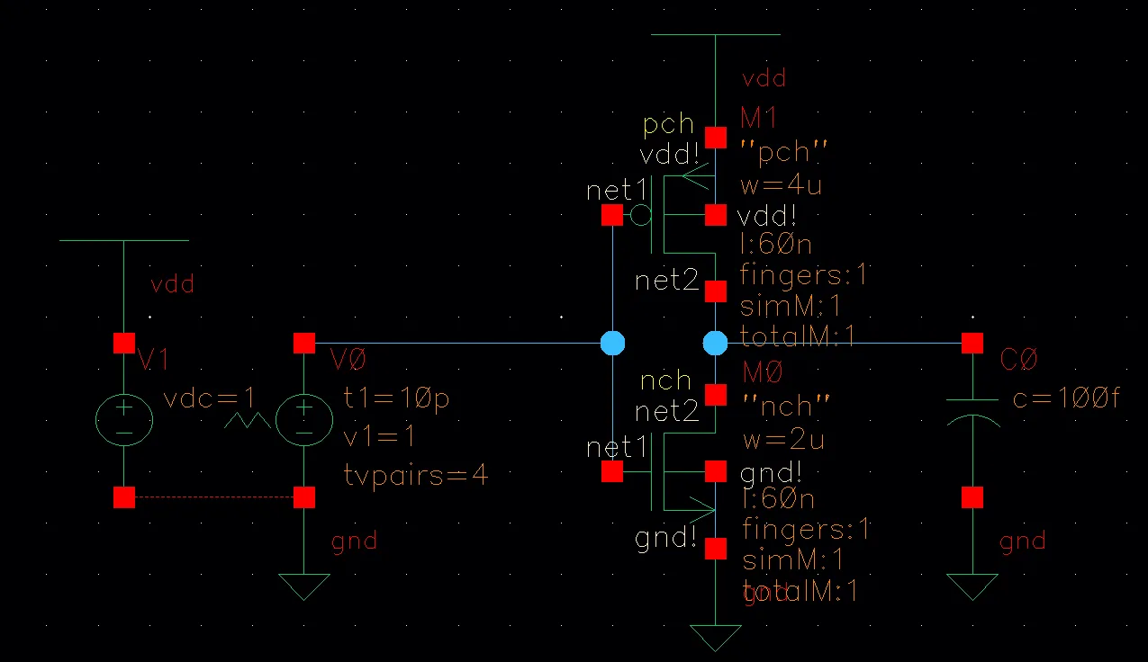
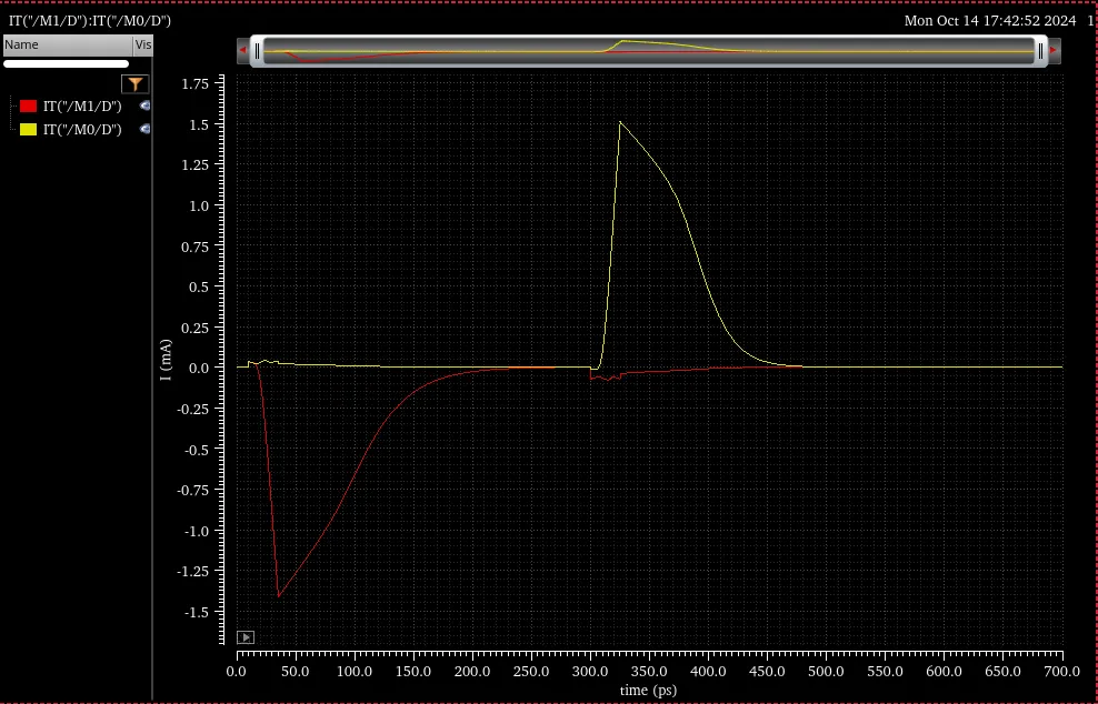
The task (HW3-2, p4–5, reconstructed from the key). An inverter (PFET 4 µm, NFET 2 µm, 60 nm, $V_{DD} = 1$ V) drives 100 fF. (a) With a 25 ps input ramp, find by simulation the energy used to charge the capacitor and the energy lost to crowbar current. (b) Repeat with a slower slew.

HW3-2, p4 (the key’s bench): a 4/2 µm inverter driving 100 fF at 1 V.

HW3-2a: a 25 ps ramp (p4–5)

HW3-2a, p4 (the key’s plot). Red: PFET drain current (negative = flowing out into the load). Yellow: NFET drain current.

Hint

Which output edge takes charge from the supply, and what is the least that charge can cost?

What it asks. By simulation, with a 25 ps input ramp: the energy used to charge the 100 fF, and the energy lost to crowbar current. That is two numbers, what the load must cost and what the circuit spends beyond it. “Crowbar” names the waste: current straight from $V_{DD}$ to ground while both devices conduct.

The idea. The bench holds the inverter (4/2 µm, 60 nm), its 100 fF load and $V_{DD} = 1$ V fixed, and sets the input ramp: 25 ps here, slower in (b). Power from a fixed supply is $V_{DD}\,i_{DD}$VDD​iDD​, so the energy the supply delivers on one edge is

$$E = \int V_{DD}\,i_{DD}\,dt = V_{DD}\int i_{DD}\,dt$$

(Chapter 6 §6). At $V_{DD} = 1$ V, femtojoules equal femtocoulombs, so the energy is the area under the supply current. The supply current flows through the PFET, so the node to watch is the PFET’s drain (or source) current, integrated over the edge. Then sort the energy by edge:

• A rising output must take $C_LV_{DD}^2$ from the supply, whatever the waveform: half is stored, half becomes heat in the PFET. Anything beyond that is waste.
• A falling output takes nothing from the supply for the load. The capacitor’s stored half becomes heat in the NFET. Any supply current on this edge is crowbar.

Crowbar current flows while the input is between $V_{Tn}$ and $V_{DD} - |V_{Tp}|$∣VTp​∣, when both devices are on (Chapter 6 §7). The tempting conclusion is that everything above $C_LV_{DD}^2$ is crowbar; the refinements after the steps say why it isn’t.

HW3-2a

1. Find the two edges on the plot. The PFET’s current charges the load and the NFET’s discharges it, so each pulse belongs to one edge. The first pulse (0–250 ps) is the rising output: the red PFET current charges the load. The yellow NFET current during it, which carries all of that edge’s crowbar, is only a blip of a few hundredths of a mA. The second pulse (300–480 ps) is the falling output: the yellow NFET discharges the load, and the small red current at its start is that edge’s crowbar.
2. Price the load. A rising output draws $C_LV_{DD}^2$ whatever the waveform: $100\,\mathrm{fF}\times(1\,\mathrm{V})^2 = 100\,\mathrm{fJ}$100fJ.
3. Read the integral. The area under the rising edge’s supply current is what the edge cost. The key’s integrated energy for the edge: about 107 fJ (reading from the key’s simulation).
4. Subtract the load. The 100 fJ is the least the edge can cost, so the rest is extra: $107 - 100 = 7\,\mathrm{fJ}$7fJ.
5. Say what the share is of. A share needs a base: $7/107 = 6.5\%$ of the edge’s total (the key’s figure), or 7% of $C_LV_{DD}^2$CL​VDD2​.

Two refinements the key skips.

• Not every edge draws 107 fJ. The key says “each transition uses a similar amount of energy”. The charge through the switching transistor is similar on both edges, but only the rising edge draws the 100 fJ from the supply; the falling edge draws only its crowbar. A full cycle costs $C_LV_{DD}^2$ plus both edges’ crowbar (Chapter 6, “Where it goes”).
• Not all of the 7 fJ is crowbar. The PFET also charges the inverter’s own drain capacitance, which the 100 fF doesn’t include. With HW3-1c’s rising-edge values, that is about $0.5 \times 4 + 0.73 \times 2 = 3.5$ fF, or about 3.5 fJ. The plot’s small NFET blip during the rising edge agrees: the true crowbar of a fast edge into a heavy load is small. The key counts the whole excess as crowbar.

Check. The excess has the right sign and size. An edge can’t draw less than $C_LV_{DD}^2$CL​VDD2​, and a fast 25 ps edge into a heavy 100 fF load should waste less than the 10–20% that Lecture 6 quotes for typical designs (Chapter 6 §7). 7% is both.

Answer: about 107 fJ per rising edge, of which 100 fJ is $C_LV_{DD}^2$ and about 7 fJ (6.5% of the total) is extra.

Remember. A simulated energy is $V_{DD}$ times the area under the supply current. Subtract $C_LV_{DD}^2$ from a rising edge to get the waste, then say what the waste is made of.

The answer key differs

Its arithmetic is right: 107 fJ, 7 fJ beyond the load, 6.5%. Two of its claims are not. “Each transition uses a similar amount of energy” holds for the charge through the switching device, but only the rising output draws the 100 fJ from the supply. And it counts all 7 fJ as crowbar, when about half of it charges the inverter’s own drains (the refinements above).

HW3-2b: a slower slew (p5)

HW3-2b, p5 (the key’s plot). The colours change: here yellow is the PFET and green the NFET.

Hint

A slower ramp keeps the input between the two thresholds for longer. Which part of the energy can that change, and which can’t it?

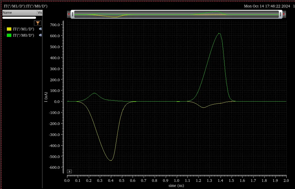
What it asks. The same measurement with a slower input ramp: the energy of the edge, and how much of it is crowbar. The key doesn’t state the slower ramp time; its plot shows edges about half a nanosecond long.

The idea. Same bench, same node and same integral as (a); the one new thing is the input’s slew, so compare the two runs part by part. $C_LV_{DD}^2$ can’t change: the supply delivers the charge $C_LV_{DD}$ at $V_{DD}$ however slowly it arrives. The inverter’s own drain capacitance costs the same too, for the same reason. Crowbar does change: both devices conduct while the input is between $V_{Tn}$ and $V_{DD} - |V_{Tp}|$∣VTp​∣, and a slower ramp keeps it there longer (Chapter 6 §7). So whatever the excess grows by is crowbar.

HW3-2b

1. Read the plot. The slower input takes longer to turn each device fully on, so the pulses now last about half a nanosecond, and the peaks drop from about 1.5 mA to about 0.6 mA. The crowbar is now plain to see: a green NFET hump of about 75 µA during the rising edge, and a yellow PFET dip of about 60 µA during the falling one. Both devices are on together for much longer.
2. Read the integral. The key’s integrated energy for the edge: 115.7 fJ (reading from the key’s simulation).
3. Subtract the load. The load still costs 100 fJ: $115.7 - 100 = 15.7\,\mathrm{fJ}$ beyond it.
4. Say what the share is of. $15.7/115.7 = 13.6\%$ of the total (the key’s figure); 15.7% of $C_LV_{DD}^2$CL​VDD2​.
5. Compare with (a). The load and the self-capacitance cost the same in both runs, so the growth is crowbar: the excess grows by $15.7 - 7 = 8.7$ fJ, to about 2.2 times (a)‘s.

Check. Two independent signs agree. The integral grew, as a slower ramp must make it, by 8.7 fJ. And the plot’s crowbar currents, blips of a few hundredths of a mA in (a), are now humps of 60–75 µA.

Answer: 115.7 fJ, so 15.7 fJ (13.6% of the total) beyond the load: roughly twice the fast edge’s excess. The self-capacitance part is the same as in (a), so the growth is crowbar. Lecture 6’s “10–20% of the dynamic power” (Chapter 6 §7) is this regime.

Remember. Slower input, more crowbar; $C_LV_{DD}^2$ never changes. When two runs differ in one setting, the difference in energy belongs to what that setting controls.

The answer key agrees

Its arithmetic is right: 15.7 fJ, 13.6%. It doesn’t state the slower ramp time.

The trend in the course model

The course’s square-law inverter (Chapter 6 §9, transient) integrates the same supply current for a ramped input. The model is not the simulator. Here it is a 1 V inverter with $V_T = \pm 0.3$ V, equal strengths and β = 6 mA/V² (chosen so the fast edge’s peak current, 1.6 mA, is close to the key’s plot), driving 100 fF, with no drain or overlap capacitance at all. Its numbers are illustrative; the trend is the point.

input ramp time (rail to rail)

100 ps

load C_L

100 fF

C_LV_DD²

100.0 fJ

supply energy, rising output

100.3 fJ

crowbar, rising output

0.25 fJ = 0.25% of that edge

crowbar, falling output

0.26 fJ

delay (50% to 50%)

59 ps

Top: the crowbar share of the supply energy on a rising-output edge, for every ramp time; the dot is the chosen ramp. Bottom: the two transistor currents on that edge. While the PFET charges the load, any NFET current goes straight from the supply to ground. Square-law devices at 1 V with V_T = ±0.3 V; no drain capacitance; not the simulator of HW3-2.

What to notice.

• The crowbar share grows steeply with the ramp time: 0.01% at 25 ps, 0.25% at 100 ps, 2.6% at 400 ps, 6.9% at 800 ps and 9.1% at 1 ns.
• At 25 ps the model’s crowbar is almost nil: the input finishes switching before the heavy load has moved, so the device turning off has almost no voltage across it. So the simulator’s 7 fJ at 25 ps is probably mostly something else, such as the self-capacitance above.
• A lighter load leaves more crowbar for the same ramp: at 400 ps, 50 fF wastes 7.4% of its $C_LV_{DD}^2$ against 2.6% for 100 fF. The output moves sooner and both devices conduct with a real voltage across them.
• The rising and falling edges waste the same here because the model’s two devices are equally strong.

Check yourself A designer halves an inverter's input ramp time. What happens to the C_LV_DD² part of the energy and to the crowbar part?

$C_LV_{DD}^2$ is unchanged: it is the charge $C_LV_{DD}$ delivered at $V_{DD}$VDD​, whatever the waveform. The crowbar part falls, because both devices are on only while the input is between $V_{Tn}$ and $V_{DD} - |V_{Tp}|$∣VTp​∣, and a faster ramp shortens that window. That is why designs set a slew-rate limit on every node.

3. HW3-3: sizing a path, then choosing the number of stages

The task (HW3-3, p6–7, reconstructed from the key). A path of three gates, a NAND, an XOR and an inverter, drives a load equal to 500 µm of gate. $C_g = 2$ fF/µm and $R_{nfet} = 4\,\mathrm{k\Omega\cdot\mu m}$4kΩ⋅μm, with $R_p = 2R_n$2Rn​. The first gate is fixed. (a) Size the other two for minimum delay and find the delay. (b) Find the number of stages that minimizes the delay, and size that path.

Reading the path. Both parts need each stage’s strength (its normalized inverter’s input) and the capacitance of its input on the path, so find them once. The handout’s gate circuits aren’t in the sources; the numbers are the key’s.

Reading HW3-3 stage by stage

1. The convention. $R_p = 2R_n$2Rn​, so the balanced inverter is 2W/W, with input $3W$3W. The unit of delay is its FO1: its NFET, $R_n/W$Rn​/W, drives the $3W\,C_g$ of an identical copy, and the widths cancel, so $\tau_{inv} = 3R_nC_g = 3 \times 4 \times 2 = 24$ ps (Chapter 7 §7).
2. Stage 1, the NAND (fixed). Its delay depends only on its strength, which the key gives as its normalized inverter, 1 µm / 0.5 µm, input 1.5 µm. It is fixed, so its own input never enters the sizing: its gain is its load over 1.5 µm, and its logical effort isn’t needed.
3. Stage 2, the XOR. The key gives its normalized inverter as $2W_2/W_2$2W2​/W2​, input $3W_2$3W2​, and its input on the path as $5W_2$5W2​. So one of its inputs loads the NAND 5/3 times as much as an inverter of the same strength would: $g = 5/3$5/3.
4. Stage 3, the inverter, $2W_3/W_3$2W3​/W3​: it is its own normalized inverter, with input $3W_3$ and $g = 1$1.
5. The load is given as 500 µm of gate, so it needs no conversion.

Stage	Gate	Normalized inverter	Input (on the path)	Logical effort
1	NAND (fixed)	1 µm / 0.5 µm, input 1.5 µm	(fixed)	(not needed)
2	XOR	$2W_2/W_2$2W2​/W2​, input $3W_2$	$5W_2$	5/3
3	inverter	$2W_3/W_3$	$3W_3$	1

HW3-3a: three stages (p6)

Hint

Write the three gains with $W_2$ and $W_3$ as unknowns and multiply them. What is left?

What it asks. Choose the XOR’s and the inverter’s sizes for the least delay, with the NAND fixed, and give that delay. Fixing the first gate fixes the path’s input capacitance. Without that you could make every gate huge and push the problem onto whatever drives the NAND.

The idea. This is the path-sizing method of M4’s path-sizing section. The new point is that the first gate is fixed and given only by its strength, so it needs no logical effort. Each stage takes $\tau_{inv}$ times its gain, and

$$\text{gain} = \frac{\text{the load the stage drives}}{\text{its normalized inverter's input}}$$ $$\text{path delay} = \tau_{inv} \sum \text{gains}$$

(Chapter 8 §1). Multiply the gains and each inner width cancels, since it appears once as a load and once as a size. That leaves the path effort $F$F, a fixed number. With a fixed product, the sum is smallest when the gains are equal: making one stage faster forces another to be slower by a larger factor (Chapter 8 §3). So every stage gets $f = F^{1/3}$F1/3; size back from the load, and let stage 1 check the work.

HW3-3a

1. Write the gains with the widths unknown. Each is what the stage drives over its own normalized input: $\dfrac{5W_2}{1.5}$1.55W2​​, $\dfrac{3W_3}{3W_2}$3W2​3W3​​, $\dfrac{500}{3W_3}$3W3​500​.
2. Multiply them. $W_2$ and $W_3$ each appear once above and once below, so they cancel: $F = \dfrac{500 \times 5}{3 \times 1.5} = 555.6$555.6. It is fixed, so equal gains minimize the sum.
3. Share it equally. Because $F$ is fixed, equal gains minimize the sum: $f = \sqrt[3]{555.6} = 8.221$8.221.
4. Size back from the load. Start at the end, because the last stage’s equation has only one unknown: $\dfrac{500}{3W_3} = f$ gives $W_3 = 20.27\,\mu$m (the inverter is $40.5/20.3\,\mu$m).
5. Then the XOR. Its gain must also be $f$f: $\dfrac{W_3}{W_2} = f$ gives $W_2 = 2.47\,\mu$m: the XOR’s normalized width. Its input is $5W_2 = 12.3\,\mu$m.
6. Let stage 1 check the work. Its gain was never set, but the three gains multiply to $F = f^3$f3, so it must come out at $f$f: $5W_2/1.5 = 12.33/1.5 = 8.22 = f$f. ✓
7. The delay. Three stages at $f$ each, with $\tau_{inv} = 3R_nC_g = 24$ ps for 2W/W inverters: $3f\,\tau_{inv} = 24.66 \times 24\,\mathrm{ps} = 591.9\,\mathrm{ps}$591.9ps.

Check. Round the widths to 2.5 and 20 µm. The gains become 8.33, 8.00 and 8.33, and the delay $24.67\,\tau_{inv}$24.67τinv​: the same to 0.02%. Near equal gains the delay is flat, so rounded widths are safe.

Answer: $W_2 = 2.47\,\mu$m, $W_3 = 20.3\,\mu$m, delay $24.7\,\tau_{inv} \approx 592$ ps. The gain of 8.2 per stage is far above the 3–4 that Chapter 8 recommends: the path has too few stages.

Remember. A fixed first gate enters only through its normalized input. Size back from the load, and stage 1’s gain checks the arithmetic.

The answer key agrees

It prints 591 ps, truncating 591.9.

HW3-3b: the best number of stages (p6–7)

Hint

Which gates can you add without changing $F$F, and what does adding one do to every stage’s gain?

What it asks. The number of stages that gives the least delay, with the three gates kept, and the sizes of that path. The words “number of stages” decide the method: $F$ stays fixed, and you choose $N$N.

The idea. The path effort is (a)‘s. An added inverter has $g = 1$ and its widths cancel like the others, so $F = 555.6$ for any $N$N. What changes is how many gains share it: each is $F^{1/N}$F1/N, and the delay is $N F^{1/N}\,\tau_{inv}$NF1/Nτinv​. More stages make every gain smaller but add one more gain to the sum; the best count is where those two effects balance. In the model that happens where every gain is $e \approx 2.72$2.72, so the best count is about $N = \ln F$ added (Chapter 8 §4). The logic limits the choice: added inverters must come in pairs, or the path’s function is inverted, so the candidates are 3, 5, 7 and 9 stages. Compare $N F^{1/N}$ for the allowed counts around $\ln F$ instead of rounding $\ln F$lnF.

HW3-3b: the stage count

1. Find the ideal count. The best gain is about $e$e, so the best count is about $N = \ln F = \ln 555.6 = 6.32$ added. Six would need three added inverters, which invert the function; look on either side, at 5 and 7.
2. Tabulate the allowed counts. Near its minimum the curve is shallow, so compare actual values: $N F^{1/N}\,\tau_{inv}$ for $N$ = 3, 5, 7 and 9 (the table below).
3. Pick the least. The question asks for the least delay, so take the smallest row: seven stages, at 414 ps. Five is only 10 ps slower: the minimum is shallow (Chapter 8 §4).

Added inverters	$N$	Gain $F^{1/N}$	Delay
0	3	8.22	$24.66\,\tau_{inv} = 592$ ps
2	5	3.54	$17.70\,\tau_{inv} = 425$ ps
4	7	2.47	$17.27\,\tau_{inv} = 414$ ps
6	9	2.02	$18.16\,\tau_{inv} = 436$ ps

Sizing seven stages. The key gives two placements of the four inverters, both with the same $f = \sqrt[7]{555.6} = 2.4666$ and the same 414 ps. Write each stage’s width as its normalized NFET width $W$ (the convention of part (a)). A stage of gain $f$ with normalized input $3W$ drives $3Wf$3Wf, so sizing back from the load gives $W_i = C_{out,i}/(3f)$Cout,i​/(3f), where $C_{out,i}$ is the next stage’s input: $3W$ for an inverter, $5W$ for the XOR.

HW3-3b: the widths

1. Start at the load. Only the last stage’s load is known: $W_7 = \dfrac{500}{3f} = 67.6\,\mu$m, in every placement.
2. (A) Both buffers between the NAND and the XOR (NAND, 4 inverters, XOR, inverter). The XOR drives the last inverter: $W_6 = \dfrac{3W_7}{3f} = 27.4\,\mu$m, input $5W_6 = 137\,\mu$m. Each inverter before it drives the next stage’s input: $W_5 = \dfrac{5W_6}{3f} = 18.5$18.5, $W_4 = 7.50$7.50, $W_3 = 3.04$3.04, $W_2 = 1.23\,\mu$m.
3. (B) One buffer before the XOR, one after it (NAND, 2 inverters, XOR, 3 inverters). The same rule: $W_6 = 27.4$27.4, $W_5 = 11.1$11.1; the XOR drives an inverter, so $W_4 = \dfrac{3W_5}{3f} = 4.50\,\mu$m, input 22.5 µm; the inverter before it drives the XOR’s $5W_4$5W4​, so $W_3 = \dfrac{5W_4}{3f} = 3.04$3.04, and $W_2 = 1.23\,\mu$m.
4. Let stage 1 check either. The seven gains multiply to $F = f^7$f7, so the NAND’s gain must come out at $f$f: $3W_2/1.5 = 3.70/1.5 = 2.47 = f$f. ✓

Where the lecture would put the inverters. Both of the key’s placements meet the 414 ps, and so does a third: all four added inverters next to the load, after the existing output inverter. That is the placement Lecture 8 calls “vastly superior from a power perspective” (Chapter 8, “Where the inverters go”): the gates near the load are the largest, so they should be inverters, not a complex gate. Here it keeps the XOR tiny:

Placement	XOR’s normalized $W$	XOR’s input (each input)	Sum of on-path inputs
(A) buffers before the XOR	27.4 µm	137 µm	431 µm
(B) one buffer each side	4.50 µm	22.5 µm	354 µm
(C) inverters at the load	0.740 µm	3.70 µm	341 µm

In (C) the widths back from the load are $67.6, 27.4, 11.1, 4.50, 1.83\,\mu$m for the five inverters and $0.740\,\mu$m for the XOR. The XOR’s other input, from off the path, must be as large as the on-path one, so placement A also loads whatever drives that input with 137 µm. The key’s two answers are correct for the delay, but (C) is the one Chapter 8 teaches.

Check. The pairing rule costs almost nothing here. Six stages, if the logic allowed them, would give 412.9 ps, only 1.5 ps below seven.

Answer: seven stages (four added inverters), each with gain $f = 2.47$2.47: $17.27\,\tau_{inv} \approx 414$ ps. Sized back from the load, the last inverter is $W_7 = 67.6\,\mu$m in every placement; the XOR is $27.4\,\mu$m with both buffers before it (A), $4.50\,\mu$m with one on each side (B), and $0.740\,\mu$m with the inverters at the load (C), the placement Chapter 8 teaches.

Remember. With $F$ fixed, more stages trade a smaller gain for one more term in the sum. Add inverters in pairs, compare $N F^{1/N}$ for the allowed counts near $\ln F$lnF, and put the added inverters next to the load.

The answer key differs

In its $n = 7$ row it writes $\sqrt[7]{555.7}\times 3\times\tau_{inv} = 414$ ps. The 555.7 and the “× 3” are typos for 555.6 and × 7: × 3 would give 178 ps. The 414 ps is right. Its other three rows are right.

The answer key differs

It gives $W_6 = \dfrac{5W_7}{3\times 2.47} = 45.53\,\mu$m “(the XOR)” in placement A, and $W_4 = 7.46\,\mu$m for the XOR in B. By part (a)‘s convention, where the XOR’s input is $5W$5W, the XOR’s widths are 27.3 µm and 4.48 µm (with the key’s rounded 2.47; 27.4 and 4.50 unrounded). The key puts the XOR’s factor 5 into the XOR’s own equation instead of the next stage’s, and then uses 3 instead of 5 in the next one; the two slips cancel. Its 45.53 and 7.46 are the XOR’s input capacitance divided by 3, so every other width in the key is right ($67.48$67.48, $18.43$18.43, $7.46$7.46, $3.02$3.02, $1.22$ and $0.99\,\mu$m with $f$ rounded to 2.47; unrounded they are 67.6, 18.5, 7.50, 3.04 and 1.23, and stage 1 comes back to exactly 1 µm).

Check yourself In HW3-3a, the first gate is fixed. Why does stage 1's gain come out equal to f without being set?

Sizing back from the load sets the gains of stages 3 and 2 to $f$f. Their product with stage 1’s gain is $F$F, which doesn’t depend on the widths, so stage 1’s gain is $F/f^2 = f$f. Checking that it does is the quickest test of the arithmetic.

What this means for the midterm

Which midterm family uses each method. The benches’ moves and traps are in How to approach a simulation-bench question; the path sizing’s in M4’s path-sizing section.

• HW3-1 (characterization) is where the exams’ $C_g$ in fF/µm, $R$ in kΩ·µm and $\tau_{inv}$ come from. Every delay question uses them as given: the chains of M3 §1–§4, MT17-3’s gate delays (M3 §7) and every path in M4. $C_d$ and $\eta$ appear in MT21-2’s FO4 (M3 §8).
• HW3-2 (energy) is the energy part of every inverter-chain question: per cycle in MT24-2a and MT23-1a (M3), per transition in MT21-4b and MT17-4c (M3). Crowbar and slew are short-answer material.
• HW3-3 (path sizing) is part (b) of MT23-5, MT21-5 and MT17-5 (M4), and the stage count is M7’s Question 5.

Traps.

• Which width goes where. Bench 1 divides by the receiving inverter’s whole gate, $8(16 + 8)$8); bench 2 divides by the 16(16/8) load and multiplies by the measured device’s width. HW3-1b’s key appears to use the wrong load and gets twice the resistance.
• Check against FO4: $12R_nC_g$ must give back the FO4 you measured.
• Energy per edge. Only a rising output draws $C_LV_{DD}^2$CL​VDD2​; a cycle is $C_LV_{DD}^2$ plus both crowbars.
• Crowbar grows with the input’s slew and shrinks with a heavier load; $C_LV_{DD}^2$ depends on neither.
• Stage counts come in steps of two. Compare $N F^{1/N}$ for the allowed $N$ around $\ln F$lnF; don’t round $\ln F$ to an even count.
• Label widths consistently. Say whether a gate’s “W” is its normalized NFET or its input over 3 (the key’s XOR mixes the two).

Time. A part like HW3-3a takes about 5 minutes on an exam; adding the stage-count table, another 3–4. The characterization and energy questions appear on midterms only as short answers or as given numbers: know what each bench measures and the one formula for each, about 2 minutes apiece.