4. Transport and the MOSFET I–V

Lecture 3 showed how a gate voltage creates a layer of electrons at the silicon surface. Lecture 4 turns that layer into a transistor: it asks how fast the electrons move, and from that derives the drain current. It does this twice, first with the classic long-channel model and then with velocity saturation, which is what real short transistors do. The second half asks why making transistors smaller made them faster for decades (Dennard scaling), and why that stopped: subthreshold leakage, short-channel effects and gate leakage.

After this chapter you can:

1. explain drift velocity, mobility and saturation velocity, with their units and typical values;
2. derive the long-channel I–V by integrating along the channel, and explain pinch-off and saturation;
3. derive the velocity-saturated I–V, find V_DSAT and I_DSAT, and say when the current becomes linear in the overdrive;
4. describe the ways a threshold voltage is measured, and translate every equation to PMOS with the right signs;
5. work out how each quantity changes under constant-field scaling, and explain the two reasons it broke down;
6. use the subthreshold slope (60 mV/decade at best) to estimate leakage, and describe DIBL, threshold roll-off and gate leakage.

Boxes and equations marked board were written in the lecture. Parts marked added are explanations or examples this guide adds.

Before you start

You need these ideas from earlier chapters. Each is restated here.

• Threshold (Chapter 3). $V_T = V_{FB} + 2\phi_F + Q_{bulk}/C_{ox}$Qbulk​/Cox​. Below $V_T$ there is no inversion layer; above it, every extra volt on the gate adds electrons to the layer.
• Oxide capacitance per area (Chapter 3). $C_{ox} = \kappa_{ox}\varepsilon_0/t_{ox}$κox​ε0​/tox​, in F/cm², with $\kappa_{ox} = 3.9$3.9.
• The inversion layer grows linearly above threshold (the Chapter 3 widget). Its charge per area is about $C_{ox}(V_{GB} - V_T)$VT​).
• Sheet versus volume quantities (Chapter 0). A charge per area (C/cm²) times a width (cm) times a velocity (cm/s) is a current (C/s = A).
• 60 mV per decade (Chapter 0). $\frac{kT}{q}\ln 10 \approx 60\,\mathrm{mV}$ at room temperature.
• Constants: $\varepsilon_0 = 8.85\times10^{-14}\,\mathrm{F/cm}$10−14F/cm, $q = 1.6\times10^{-19}\,\mathrm{C}$10−19C, $kT/q = 26\,\mathrm{mV}$26mV.

Notation. $V_T$ is the threshold voltage; the thermal voltage is always written $kT/q$kT/q. The electric field is $\mathcal{E}$E, as on the board. $W$ and $L$ are the transistor’s width and channel length (Chapter 3).

One device for the examples. added The worked examples use one illustrative NMOS, not a fit to a real process: $W = 1\,\mu\mathrm{m}$1μm, $t_{ox} = 5.4\,\mathrm{nm}$ (the lecture’s oxide for the 0.25 µm generation, 70:39), $\mu = 400\,\mathrm{cm^2/V\cdot s}$400cm2/V⋅s, $v_{sat} = 10^7\,\mathrm{cm/s}$107cm/s, $V_T = 0.5\,\mathrm{V}$0.5V, and $V_{GS} = 2.5\,\mathrm{V}$2.5V, the supply of that generation. It comes in two lengths, $L = 10\,\mu\mathrm{m}$ and $L = 0.25\,\mu\mathrm{m}$0.25μm.

1. Drift velocity and mobility

The idea. Carriers in silicon move fast but randomly. A field adds a small net velocity, the drift velocity, which is proportional to the field at low fields and levels off at the saturation velocity at high fields.

Random motion, and drift

Picture an electron (or a hole) in silicon (01:10–02:24). It moves at the thermal velocity, set by its thermal energy, and keeps scattering, changing direction at random. With no field, all that motion goes nowhere on average.

Apply a field $\mathcal{E}$ and each carrier still bangs around randomly, but between collisions the field pushes it a little in one direction. On average the cloud picks up a net velocity: the drift velocity $v_{drift}$ (02:09). Holes drift along the field; electrons, being negative, drift against it.

This picture, carriers that scatter many times on their way, is diffusive transport. The lecturer warns at the start (00:42) that in very short modern transistors the carriers cross from source to drain with hardly any scattering. That is ballistic or quasi-ballistic transport. The diffusive picture used here is still the right starting point, because its main ideas carry over (01:10).

Press Play to watch it. Start with no field, then raise it.

PlayShow holes

electric field ℰ

2.0 kV/cm

carriers

electrons (drift against ℰ)

v_drift = μℰ

8.00×10⁵ cm/s

thermal velocity

~1.0×10⁷ cm/s

v_drift / v_thermal

0.080

One carrier leaves a trail. Each carrier moves at the thermal speed and changes direction at every scattering event. Between events the field speeds it up a little in one direction, so on average the cloud drifts. The drift is drawn 3× larger than its true share of the thermal motion; even so, at a few kV/cm it is a small bias on a random walk.

What to notice.

• With $\mathcal{E} = 0$ the carriers wander, and the marked one’s trail goes nowhere in particular.
• With a field, every path still zigzags, but the cloud slowly slides one way. Switch to holes and it slides the other way.
• Even at 5 kV/cm, $v_{drift}$ is only a fifth of the thermal speed. Drift is a small bias on a fast random motion.

Mobility

Lecture04 @ 05:29Drift velocity against field: slope μ at low field, flattening at v_sat (top right: the saturation velocities).

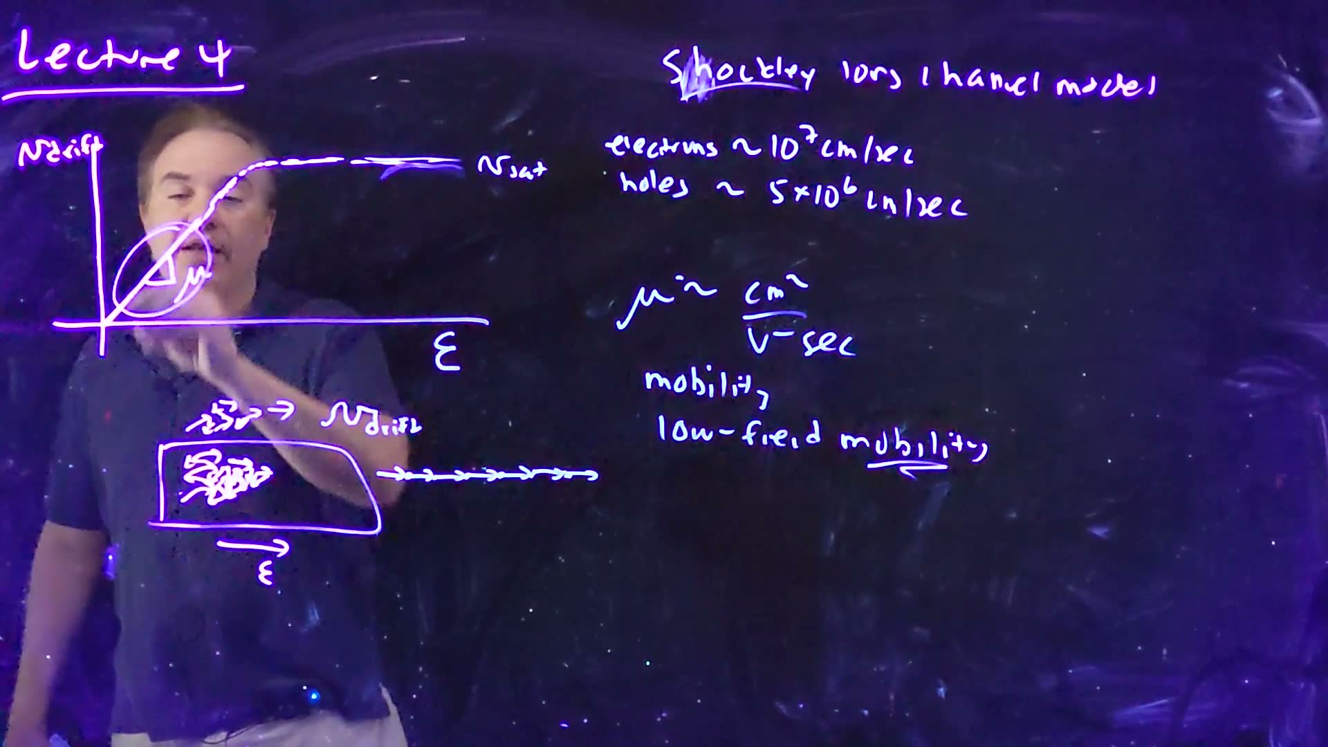
At low fields the drift velocity is proportional to the field (02:24):

$$v_{drift} = \mu\mathcal{E} .$$

The constant $\mu$ is the mobility, the slope of the curve on the board. Its units follow from the equation: (cm/s)/(V/cm) = cm²/V·s (02:41). You will also hear “low-field mobility”. The lecturer finds that redundant, since mobility is by definition a low-field quantity.

Saturation velocity

The line can’t go on forever (03:07). If the field were so strong that carriers went straight forward after every collision, the drift velocity would be limited to about the thermal velocity. That is what happens: the curve flattens at the saturation velocity $v_{sat}$vsat​, and the effect is called velocity saturation (03:38). On the board:

• electrons: $v_{sat} \sim 10^7\,\mathrm{cm/s}$107cm/s;
• holes: about half that, $\sim 5\times10^6\,\mathrm{cm/s}$106cm/s.

In quasi-ballistic modern devices the curve has the same shape, but the ceiling is the source injection velocity, the speed at which carriers leave the source: a few times $10^7\,\mathrm{cm/s}$107cm/s, about the fastest carriers get in silicon devices (04:39).

The plan for the rest of the lecture follows from this curve: first the Shockley long-channel model, which assumes $v_{drift} = \mu\mathcal{E}$ everywhere, then a model with velocity saturation (05:11).

Worked example. added With $\mu = 400\,\mathrm{cm^2/V\cdot s}$400cm2/V⋅s:

1. At $\mathcal{E} = 1\,\mathrm{kV/cm} = 10^3\,\mathrm{V/cm}$103V/cm: $v_{drift} = 400 \times 10^3 = 4\times10^5\,\mathrm{cm/s}$105cm/s.
2. At $10^5\,\mathrm{V/cm}$ the straight line would give $4\times10^7\,\mathrm{cm/s}$107cm/s, four times the electron saturation velocity. The line has stopped being true long before that field.
3. For scale: 2 V across a 10 µm channel is a field of $2\times10^3\,\mathrm{V/cm}$103V/cm; 2 V across 0.25 µm is $8\times10^4\,\mathrm{V/cm}$104V/cm. Short channels are where velocity saturation matters.

Common mistakes.

• Writing mobility in m²/V·s and mixing it with cm-based doping and capacitance. Device physics uses cm throughout (Chapter 0).
• Thinking a carrier moves at $v_{drift}$vdrift​. Its actual speed is the much larger thermal velocity; $v_{drift}$ is the average of a random motion.

Check yourself Electrons have v_sat ≈ 10⁷ cm/s and holes about half. Which carrier makes the faster transistor of the same size, and by roughly how much at high fields?

Electrons. When the carriers are velocity-saturated, the current is proportional to $v_{sat}$ (Section 7), so an NMOS carries about twice the current of an equal PMOS. That is one reason PMOS devices are drawn wider (a later lecture).

2. The channel current: charge times velocity

The idea. The drain current is the inversion-layer charge swept along by the drift velocity: width × charge per area × velocity.

Lecture04 @ 13:21The long-channel derivation: the device and V(x) (left), then I_D = W Q_i(x) v_drift and the integral (right). The right end runs off the frame.

The setup

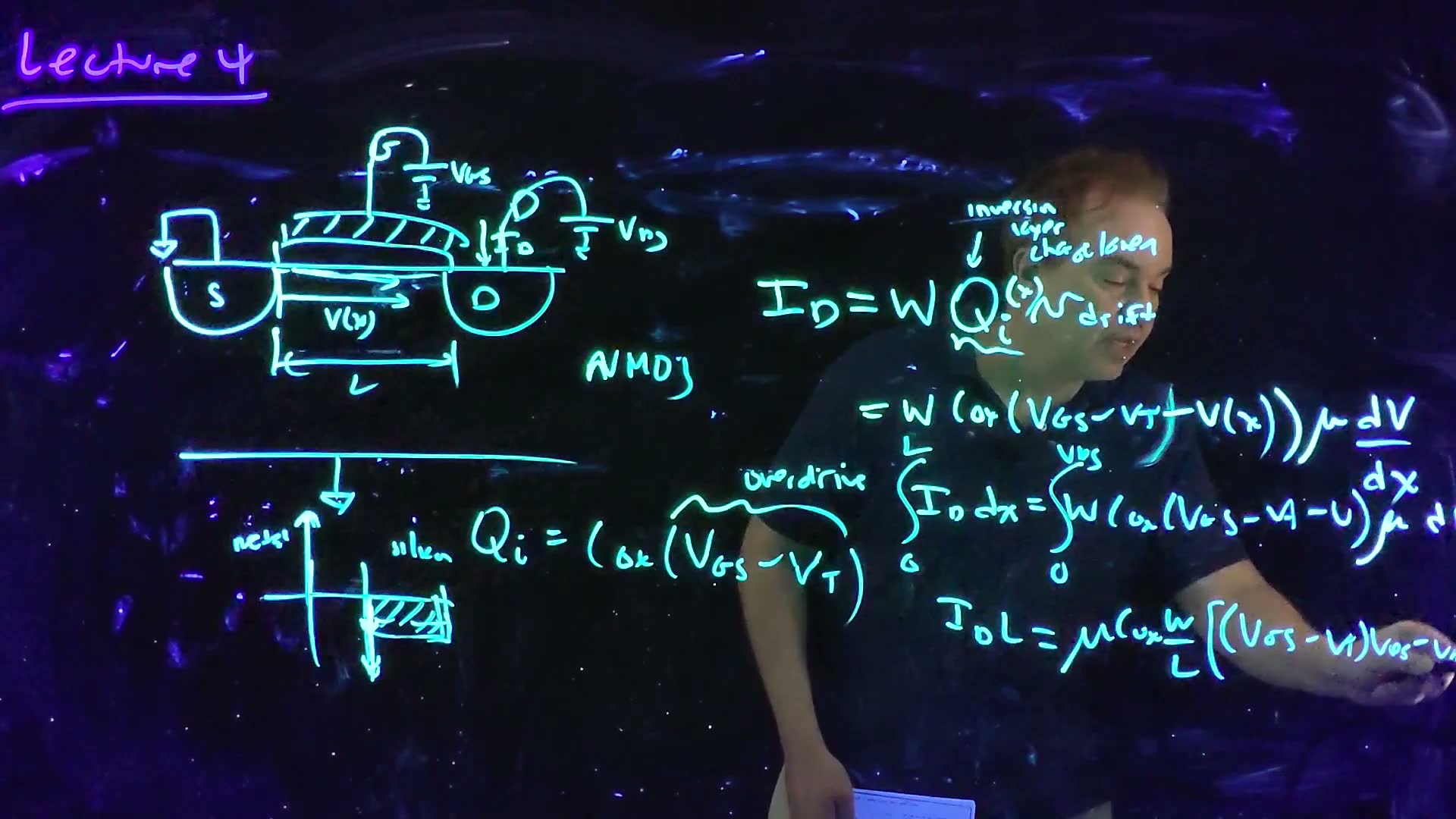
The lecture analyses an NMOS (06:36–08:03):

• the source and body are grounded, so they sit at the same potential. When they don’t, the threshold changes; that is the body effect, in Lecture 5 (Chapter 5);
• a voltage $V_{GS}$ on the gate and $V_{DS}$ on the drain;
• electrons flow from source to drain, so the conventional current, which by Benjamin Franklin’s convention flows the way positive charge would, flows from drain to source (07:32). $I_D$ is that current, flowing into the drain.

Let $x$ run along the channel from the source ($x = 0$x=0) to the drain ($x = L$x=L), and let $V(x)$ be the channel potential at $x$x, from $V(0) = 0$ to $V(L) = V_{DS}$ (08:05).

The current equation

At any point along the channel, the current is the charge passing per second (08:29):

Channel currentboard

$$I_D = W\,Q_i(x)\,v_{drift}(x)$$

$Q_i$ is the inversion-layer charge per area (its size; the electrons’ charge is negative), $W$ the width, $v_{drift}$ the electrons’ drift velocity.

Holds when: steady state; the same current flows through every cross-section of the channel

Check the units (08:59): $\mathrm{cm} \times \mathrm{C/cm^2} \times \mathrm{cm/s} = \mathrm{C/s}$C/s, a current. In words: each second the electrons sweep out a strip of inversion charge $v_{drift}$ long and $W$ wide (09:25). So the current can rise in only two ways: more charge, or faster charge.

A note on signs. added The lecturer is “a little bit lax with minus signs” (26:13). The equations here use sizes: $Q_i$Qi​, $\mathcal{E}$ and $v_{drift}$ are all positive, and $I_D$ is positive into the drain. Electrons actually move toward the drain while the field points toward the source, and the two signs cancel.

3. Inversion charge and overdrive

The idea. Once the gate is past threshold, every extra volt across the oxide adds $C_{ox}$ worth of electrons per area. Along the channel, the voltage across the oxide shrinks toward the drain, and so does the charge.

At the source end the channel is at 0 V, and the gate sees the full $V_{GS}$ (09:52). Up to threshold, gate voltage only deepens the depletion region (Chapter 3). Beyond threshold, all the extra gate voltage appears across the oxide, as a capacitor with gate charge on one side and inversion electrons on the other (10:46):

$$Q_i = C_{ox}\,(V_{GS} - V_T) .$$

The excess $V_{GS} - V_T$ is the overdrive (11:14): how far beyond threshold the device is driven. More overdrive, more inversion charge, more current.

Along the channel

The channel is not at 0 V everywhere. At a point $x$ it sits at $V(x)$V(x), so the gate-to-channel voltage there is $V_{GS} - V(x)$V(x), and the overdrive there is $V_{GS} - V_T - V(x)$ (11:53–12:20):

Inversion charge along the channelboard

$$Q_i(x) = C_{ox}\,\bigl(V_{GS} - V_T - V(x)\bigr)$$

At the source, $C_{ox}(V_{GS} - V_T)$VT​). At the drain, $C_{ox}(V_{GS} - V_T - V_{DS})$VDS​): less charge.

Holds when: strong inversion everywhere along the channel; V_T taken the same at every point

Worked example. added The chapter’s device at the source end, $V_{GS} - V_T = 2\,\mathrm{V}$2V.

1. $C_{ox} = \kappa_{ox}\varepsilon_0/t_{ox} = 3.9 \times 8.854\times10^{-14}/(5.4\times10^{-7}) = 6.39\times10^{-7}\,\mathrm{F/cm^2}$10−7F/cm2.
2. $Q_i = C_{ox}(V_{GS} - V_T) = 6.39\times10^{-7} \times 2 = 1.28\times10^{-6}\,\mathrm{C/cm^2}$10−6C/cm2.
3. As electrons: $Q_i/q = 1.28\times10^{-6}/1.602\times10^{-19} = 7.98\times10^{12}$ electrons per cm². This is a sheet: compare it with Chapter 3’s depletion charge, $Q_{bulk} = 1.66\times10^{-7}\,\mathrm{C/cm^2}$10−7C/cm2, about $10^{12}$ ions per cm².

Check yourself The overdrive is 2 V at the source and V_DS = 1.5 V. What fraction of the source-end charge is left at the drain end?

At the drain the overdrive is $2 - 1.5 = 0.5\,\mathrm{V}$0.5V, so $Q_i$ is a quarter of its source value.

4. The long-channel I–V and saturation

The idea. With $v_{drift} = \mu\, dV/dx$μdV/dx, the current equation can be integrated along the channel. The result is a parabola in $V_{DS}$VDS​. Its top is where the channel pinches off at the drain, and beyond that point the current stays flat.

Integrate along the channel

Long-channel (Shockley) current (board, 12:20–13:16)

1. Substitute $Q_i(x)$ and $v_{drift} = \mu\mathcal{E} = \mu\,\dfrac{dV}{dx}$ board: $I_D = W C_{ox}\bigl(V_{GS} - V_T - V(x)\bigr)\,\mu\dfrac{dV}{dx}$V(x))μdxdV​.
2. Multiply both sides by $dx$dx. $I_D$ is the same at every $x$x, so it can come out of the integral on the left added.
3. Integrate $x$ from 0 to $L$L, and $V$ from $0$ to $V_{DS}$ board: $\displaystyle\int_0^L I_D\,dx = \int_0^{V_{DS}} W C_{ox}\mu\,(V_{GS} - V_T - V)\,dV$V)dV.
4. The left side is $I_D L$ID​L. The right side is $W C_{ox}\mu\left[(V_{GS} - V_T)V_{DS} - \dfrac{V_{DS}^2}{2}\right]$WCox​μ[(VGS​−VT​)VDS​−2VDS2​​].
5. Divide by $L$ board: $I_D = \mu C_{ox}\dfrac{W}{L}\left[(V_{GS} - V_T)V_{DS} - \dfrac{V_{DS}^2}{2}\right]$μCox​LW​[(VGS​−VT​)VDS​−2VDS2​​].

The board’s last line still reads "$I_D L =$" with $W/L$ on the right; the lecturer catches it (13:16): the $L$ has already moved over. The board’s right end also runs off the camera frame, where $V_{DS}^2/2$ completes it.

A parabola, and pinch-off

Lecture04 @ 20:48The parabola, pinch-off at the drain end, and the flat saturation current.

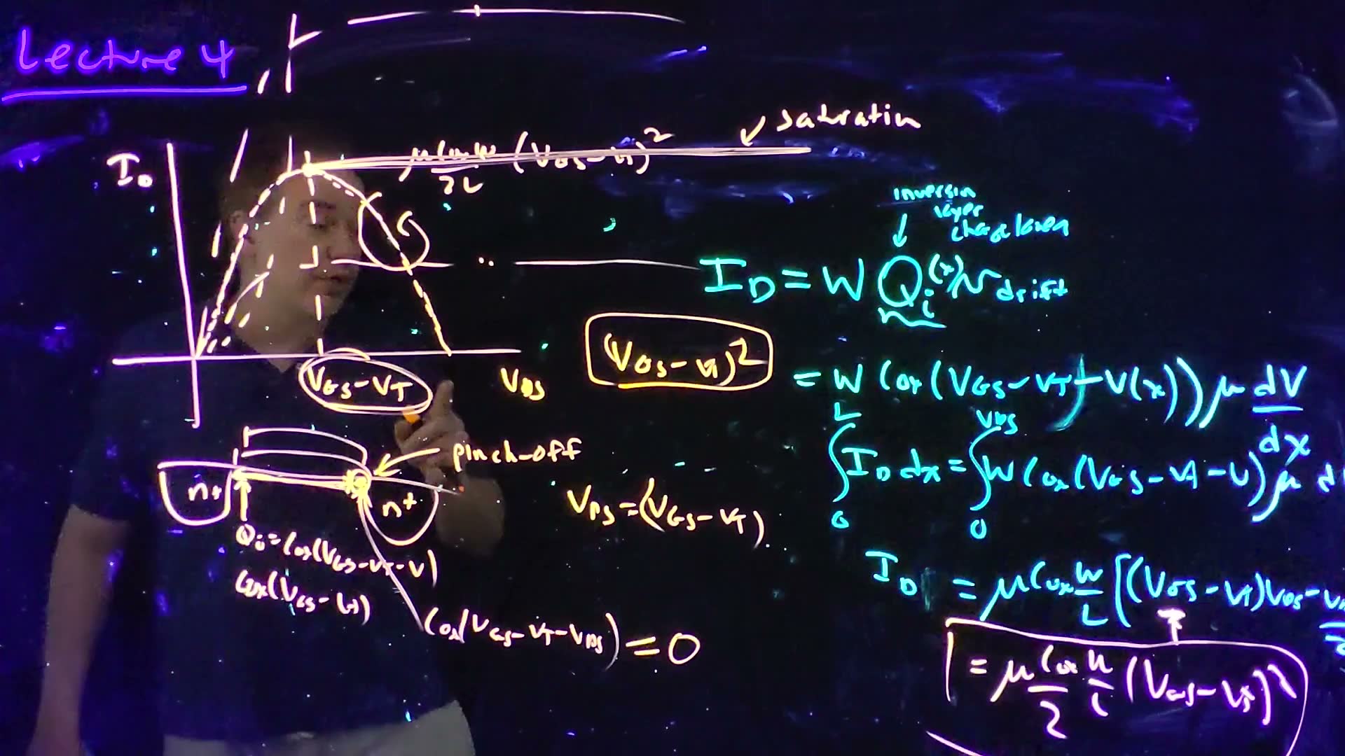
Fix $V_{GS}$ and plot $I_D$ against $V_{DS}$ (14:45). The formula is a downward parabola. Its peak is where $dI_D/dV_{DS} = 0$0:

The top of the parabola (board, 15:14–15:40)

1. Differentiate added: $\dfrac{dI_D}{dV_{DS}} = \mu C_{ox}\dfrac{W}{L}\bigl[(V_{GS} - V_T) - V_{DS}\bigr]$VDS​].
2. It is zero at $V_{DS} = V_{GS} - V_T$ board.
3. Substitute back: $(V_{GS} - V_T)^2 - \tfrac12(V_{GS} - V_T)^2 = \tfrac12(V_{GS} - V_T)^2$VT​)2, so the peak current is $\mu C_{ox}\dfrac{W}{2L}(V_{GS} - V_T)^2$ board.

Past the peak the parabola falls, which “really doesn’t make a lot of sense” (16:05): more drain voltage, less current? Go back to the charge. At the drain end, $Q_i(L) = C_{ox}(V_{GS} - V_T - V_{DS})$VDS​). When $V_{DS} = V_{GS} - V_T$VT​, this is zero: the inversion layer has vanished at the drain end. This is pinch-off (17:01–17:25).

Saturation

What happens if $V_{DS}$ rises further (17:25–18:56)?

• The channel itself still only holds $V_{GS} - V_T$ from source to pinch-off point; that voltage is now fixed.
• The extra $V_{DS} - (V_{GS} - V_T)$ drops across the short pinched-off region next to the drain, a depleted region that electrons cross rapidly once they reach it.
• The current is set by transport through the part of the channel that is not pinched off, which sees a fixed voltage. So the current stops changing: it saturates. It doesn’t fall as the parabola would say; it flatlines at the peak value.

Long-channel (Shockley) modelboard

$$\beta = \mu C_{ox}\frac{W}{L}$$

Triode, for $V_{DS} < V_{GS} - V_T$VT​:

$$I_D = \beta\left[(V_{GS} - V_T)V_{DS} - \frac{V_{DS}^2}{2}\right]$$

Saturation, for $V_{DS} \ge V_{DSAT} = V_{GS} - V_T$VT​:

$$I_{DSAT} = \frac{\beta}{2}\,(V_{GS} - V_T)^2$$

The board writes $\mu C_{ox}W/L$ out in full; the shorthand $\beta$ is added.

Holds when: v_drift = μℰ everywhere (no velocity saturation); V_GS > V_T; source and body at the same potential

Names of the two regions (37:43–38:19). The rising part, where the current is roughly linear in $V_{DS}$VDS​, is the linear or triode region. “Triode” refers to vacuum-tube triodes, whose characteristics looked like this part: a variable resistor. The flat part is the saturation region.

Raising $V_{GS}$ gives a family of curves, each saturating at its own $V_{DS} = V_{GS} - V_T$VT​, with saturated currents growing as the square of the overdrive (19:22). That matters because digital circuits work by charging and discharging capacitors, and most of that work is done by transistors in saturation (19:49). The saturation current sets switching speed.

Worked example. added The long device, $L = 10\,\mu\mathrm{m}$10μm, at $V_{GS} = 2.5\,\mathrm{V}$ (overdrive 2 V).

1. $\mu C_{ox} = 400 \times 6.39\times10^{-7} = 2.56\times10^{-4}\,\mathrm{A/V^2}$10−4A/V2, and $\mu C_{ox}W/L = 2.56\times10^{-4}/10 = 2.56\times10^{-5}\,\mathrm{A/V^2}$10−5A/V2.
2. $V_{DS} = 0.1\,\mathrm{V}$ (triode): $I_D = 2.56\times10^{-5}\,[2(0.1) - 0.1^2/2] = 2.56\times10^{-5} \times 0.195 = 4.99\,\mu\mathrm{A}$4.99μA.
3. $V_{DS} = 1\,\mathrm{V}$ (triode): $I_D = 2.56\times10^{-5}\,[2 - 0.5] = 38.4\,\mu\mathrm{A}$38.4μA.
4. $V_{DSAT} = 2\,\mathrm{V}$2V: $I_{DSAT} = \tfrac12 \times 2.56\times10^{-5} \times 2^2 = 51.2\,\mu\mathrm{A}$51.2μA.
5. $V_{DS} = 3\,\mathrm{V}$3V: still $51.2\,\mu\mathrm{A}$51.2μA, since the device is saturated.

Common mistakes.

• Using the triode formula past $V_{DSAT}$VDSAT​. Check the region first: is $V_{DS}$ below or above $V_{GS} - V_T$VT​?
• Thinking pinch-off stops the current. The current is set by the channel; the pinched-off region just carries it to the drain.

Check yourself In saturation, V_GS − V_T is doubled from 1 V to 2 V. By what factor does the long-channel I_DSAT grow? And V_DSAT?

$I_{DSAT} \propto (V_{GS} - V_T)^2$ grows 4×. $V_{DSAT} = V_{GS} - V_T$ doubles.

5. Why the current goes as the square of the overdrive

The idea. The overdrive enters twice: once in how much charge there is, and once in how fast it moves.

Lecture04 @ 22:48The two factors of the overdrive: Q_i, and v_drift through ℰ ~ V_DS/L.

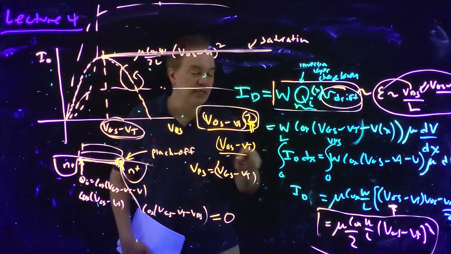
Go back to $I_D = W Q_i v_{drift}$ (20:35–21:54):

1. Charge. $Q_i = C_{ox}(V_{GS} - V_T)$VT​): one factor of the overdrive.
2. Velocity. $v_{drift} = \mu\mathcal{E}$μE, and the field is roughly $V_{DS}/L$VDS​/L. In saturation $V_{DS}$ is $V_{GS} - V_T$VT​, so a larger overdrive means a larger field, a faster drift: the second factor.

“If this were true today, … we would have very, very fast microprocessors” (21:54). It isn’t, because the drift velocity saturates. Then the velocity factor stops growing with the field, and the current is left with only the charge factor: linear in the overdrive (22:22). Sections 6 and 7 show this properly.

Check yourself Which of the two factors does velocity saturation remove, and why?

The velocity factor. Once the field is high, $v_{drift}$ is stuck near $v_{sat}$vsat​, so raising the overdrive no longer makes the carriers faster. It still adds charge, so the current still grows, but only linearly.

6. Velocity saturation: a model for the drift velocity

The idea. A simple formula, $v_{drift} = \mu\mathcal{E}/(1 + \mathcal{E}/\mathcal{E}_{crit})$E/Ecrit​), follows $\mu\mathcal{E}$ at low fields and flattens at $v_{sat} = \mu\mathcal{E}_{crit}$ at high fields.

The lecture now redoes the derivation with velocity saturation. It follows Taur and Ning’s textbook (on the course reserves), which goes through it in more detail, and the problem set has you plot the results (23:16–23:35).

Velocity-saturation modelboard

$$v_{drift} = \frac{\mu\mathcal{E}}{1 + \mathcal{E}/\mathcal{E}_{crit}}, \qquad v_{sat} = \mu\,\mathcal{E}_{crit}$$

$\mathcal{E}_{crit}$ is the critical electric field, typically about $10^4\,\mathrm{V/cm}$ (25:13).

Holds when: phenomenological: a curve fit, used in SPICE models, not derived from physics

“The first time I saw this expression, I thought there was some deep physics … This is nothing more than a curve fit” (24:46). It is the curve the SPICE models use.

The two limits (board, 25:13)

1. Low field, $\mathcal{E} \ll \mathcal{E}_{crit}$Ecrit​: the denominator is about 1, so $v_{drift} = \mu\mathcal{E}$μE, the mobility line.
2. High field, $\mathcal{E} \gg \mathcal{E}_{crit}$Ecrit​: the denominator is about $\mathcal{E}/\mathcal{E}_{crit}$E/Ecrit​, so $v_{drift} = \mu\mathcal{E}\cdot\mathcal{E}_{crit}/\mathcal{E} = \mu\mathcal{E}_{crit}$μEcrit​, a constant.
3. That constant is the saturation velocity: $v_{sat} = \mu\mathcal{E}_{crit}$μEcrit​.

mobility μ

400 cm²/V·s

saturation velocity v_sat

1.0×10⁷ cm/s

ℰ_crit = v_sat/μ

25.0 kV/cm

fit at ℰ_crit

5.00×10⁶ cm/s = v_sat/2

at 10 kV/cm: μℰ

4.00×10⁶ cm/s

at 10 kV/cm: fit

2.86×10⁶ cm/s (71%)

The fit is the lecture's curve (24:27): it follows μℰ at low field and flattens to v_sat = μℰ_crit at high field. At ℰ = ℰ_crit it is only halfway there.

What to notice.

• At $\mathcal{E} = \mathcal{E}_{crit}$ the fit gives exactly $v_{sat}/2$ added, and $\mu\mathcal{E}$ gives $v_{sat}$vsat​. The critical field marks the middle of the bend, not where saturation is complete.
• Raising $\mu$ at fixed $v_{sat}$ lowers $\mathcal{E}_{crit} = v_{sat}/\mu$vsat​/μ: high-mobility carriers saturate at lower fields.

Worked example. added The chapter’s values, $\mu = 400$ and $v_{sat} = 10^7\,\mathrm{cm/s}$107cm/s.

1. $\mathcal{E}_{crit} = v_{sat}/\mu = 10^7/400 = 2.5\times10^4\,\mathrm{V/cm}$104V/cm, “on the order of $10^4$104”.
2. At $\mathcal{E} = 10^4\,\mathrm{V/cm}$104V/cm: $v_{drift} = 400\times10^4/(1 + 0.4) = 2.86\times10^6\,\mathrm{cm/s}$106cm/s, 71% of $\mu\mathcal{E}$μE.
3. The lecture’s check the other way round (25:49): $\mathcal{E}_{crit} \approx 10^4\,\mathrm{V/cm}$ with typical mobilities gives $v_{sat}$ near $10^7\,\mathrm{cm/s}$107cm/s.

7. The velocity-saturated I–V

The idea. Put the new drift velocity into the same current equation and integrate again. The current is the long-channel current divided by a factor that grows with $V_{DS}/L$VDS​/L. It saturates earlier and lower, and for short channels it becomes linear in the overdrive.

Lecture04 @ 33:04The velocity-saturated derivation, V_DS,sat, I_D,sat and the high-field limit.

The current

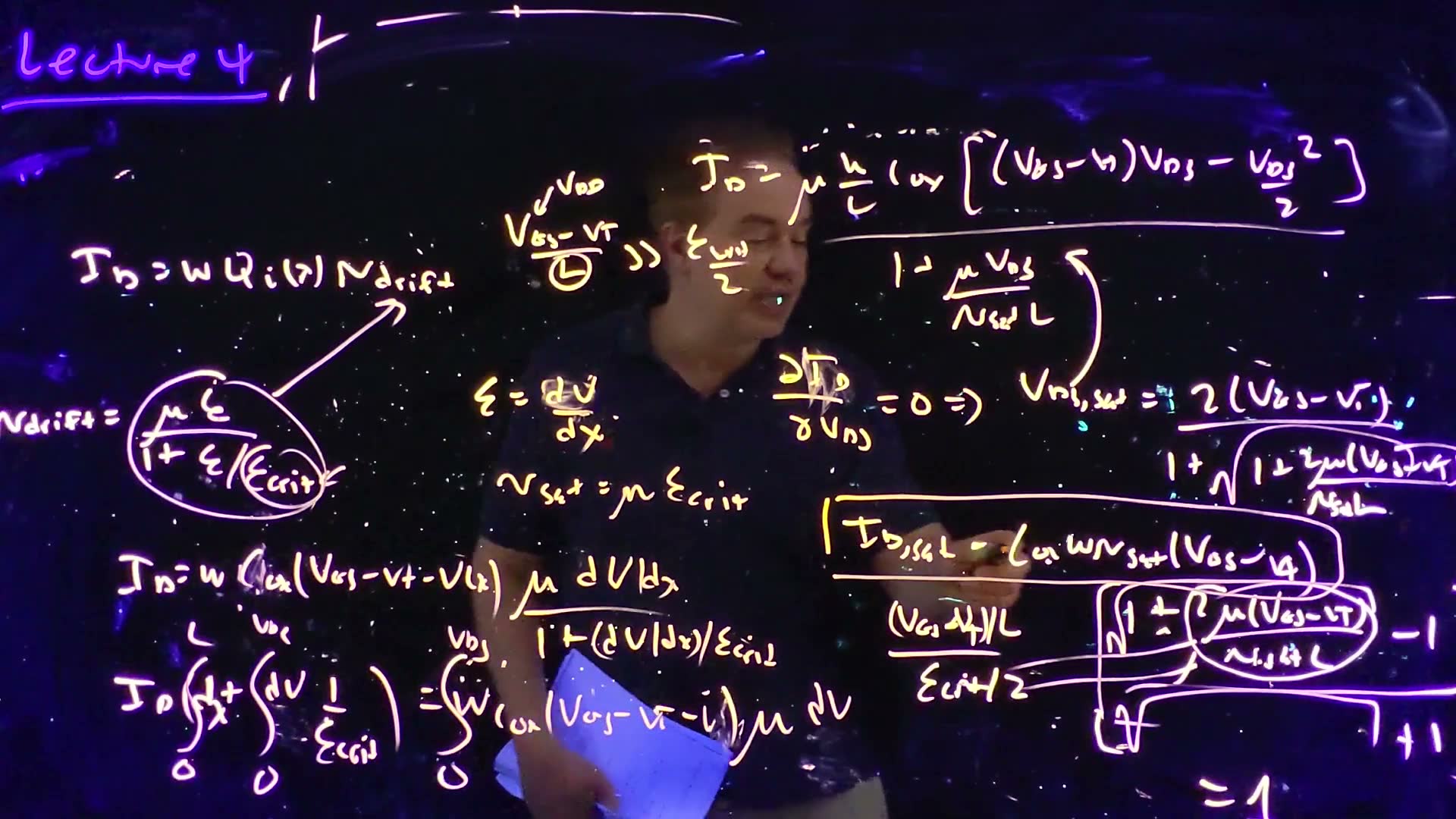
Velocity-saturated current (board, 25:49–28:54)

1. Start again from $I_D = W Q_i(x)\,v_{drift}$WQi​(x)vdrift​, with $\mathcal{E} = dV/dx$ board: $I_D = W C_{ox}\bigl(V_{GS} - V_T - V\bigr)\,\dfrac{\mu\,dV/dx}{1 + (dV/dx)/\mathcal{E}_{crit}}$V)1+(dV/dx)/Ecrit​μdV/dx​.
2. Multiply both sides by the denominator added: $I_D\Bigl(1 + \dfrac{1}{\mathcal{E}_{crit}}\dfrac{dV}{dx}\Bigr) = W C_{ox}\mu\,(V_{GS} - V_T - V)\dfrac{dV}{dx}$V)dxdV​.
3. Multiply by $dx$ and integrate, $x$ from 0 to $L$ and $V$ from 0 to $V_{DS}$ board: $I_D\Bigl(\displaystyle\int_0^L dx + \int_0^{V_{DS}}\frac{dV}{\mathcal{E}_{crit}}\Bigr) = \int_0^{V_{DS}} W C_{ox}\mu\,(V_{GS} - V_T - V)\,dV$V)dV.
4. The left side is $I_D\,(L + V_{DS}/\mathcal{E}_{crit})$VDS​/Ecrit​). The right side is the same integral as Section 4.
5. Divide by $L$L, and write $1/\mathcal{E}_{crit} = \mu/v_{sat}$ board: $I_D = \dfrac{\mu C_{ox}\frac{W}{L}\Bigl[(V_{GS} - V_T)V_{DS} - \frac{V_{DS}^2}{2}\Bigr]}{1 + \dfrac{\mu V_{DS}}{v_{sat}L}}$1+vsat​LμVDS​​μCox​LW​[(VGS​−VT​)VDS​−2VDS2​​]​.

The numerator is exactly the long-channel current. The denominator is $1 + V_{DS}/(\mathcal{E}_{crit}L)$VDS​/(Ecrit​L): the average field $V_{DS}/L$ compared with $\mathcal{E}_{crit}$Ecrit​. When the field is small, the denominator is about 1 and the two models agree.

Saturation voltage and current

This curve is also “parabolic-ish” with a maximum (29:00). Set $\partial I_D/\partial V_{DS} = 0$0. Write $U = V_{GS} - V_T$ and $b = \mu/(v_{sat}L)$ for short added:

Saturation voltage (board, 29:00–30:09)

1. $I_D \propto \dfrac{UV - V^2/2}{1 + bV}$1+bVUV−V2/2​. By the quotient rule, the slope is zero when $(U - V)(1 + bV) - b\,(UV - V^2/2) = 0$0.
2. Expand: $U - V + bUV - bV^2 - bUV + \tfrac12 bV^2 = 0$0, that is, $\tfrac12 bV^2 + V - U = 0$0.
3. Solve the quadratic for the positive root: $V = \dfrac{-1 + \sqrt{1 + 2bU}}{b}$b−1+1+2bU​​.
4. Multiply top and bottom by $1 + \sqrt{1 + 2bU}$1+2bU​: $V_{DSAT} = \dfrac{2U}{1 + \sqrt{1 + 2bU}}$ board, with $2bU = \dfrac{2\mu(V_{GS} - V_T)}{v_{sat}L}$vsat​L2μ(VGS​−VT​)​.

Watch out at 29:46. The lecturer first writes the term under the root as “two μ (V_GS − V_T) over L”, then corrects himself on units: “I think this has to be v_sat L, actually” (29:58). The board has $v_{sat}L$vsat​L. Check it: $\mu(V_{GS} - V_T)/(v_{sat}L)$ has units (cm²/V·s)(V)/((cm/s)(cm)) = 1, dimensionless, as it must be.

Put $V_{DSAT}$ back into $I_D$ to get the saturation current (30:39). The lecturer calls it “an ugly equation”; a shorthand makes it readable.

Velocity-saturated modelboard

Triode, for $V_{DS} < V_{DSAT}$VDSAT​:

$$I_D = \frac{I_{D,\text{long}}}{1 + \dfrac{\mu V_{DS}}{v_{sat}L}}$$$$s = \sqrt{1 + \frac{2\mu\,(V_{GS} - V_T)}{v_{sat}L}}$$$$V_{DSAT} = \frac{2\,(V_{GS} - V_T)}{1 + s}$$$$I_{DSAT} = C_{ox}Wv_{sat}\,(V_{GS} - V_T)\,\frac{s - 1}{s + 1}$$

$I_{D,\text{long}}$ is the long-channel triode current of Section 4. The shorthand $s$ is added; the board writes the square root out.

Holds when: v_drift = μℰ/(1 + ℰ/ℰ_crit); V_GS > V_T; flat (saturated) for V_DS ≥ V_DSAT

The short-channel limit

Since $\mu/v_{sat} = 1/\mathcal{E}_{crit}$1/Ecrit​, the term under the root compares a field with the critical field (31:21–32:05):

$$\frac{2\mu(V_{GS} - V_T)}{v_{sat}L} = \frac{(V_{GS} - V_T)/L}{\mathcal{E}_{crit}/2} .$$

The largest $V_{GS}$ is the supply, $V_{DD}$VDD​, and $L$ is the channel length. As $L$ shrinks, $(V_{GS} - V_T)/L$ grows (32:37). When it is much larger than $\mathcal{E}_{crit}/2$Ecrit​/2, $s$ is large, $(s - 1)/(s + 1) \to 1$1, and (33:03):

Fully velocity-saturated currentboard

$$I_{DSAT} = C_{ox}\,W\,v_{sat}\,(V_{GS} - V_T)$$

Linear in the overdrive, and independent of $L$ and $\mu$μ.

Holds when: (V_GS − V_T)/L ≫ ℰ_crit/2: short channels, 0.25 µm and below

This reads straight off $I_D = W Q_i v$ added: charge $C_{ox}(V_{GS} - V_T)$VT​), moving at $v_{sat}$vsat​. The lecturer says the criterion holds for quarter-micron technologies and below (34:19): from then on, transistors behave velocity-saturated.

The other limit. added For a long channel, $2bU$ is small and $s = \sqrt{1 + 2bU} \approx 1 + bU$bU. Then $(s - 1)/(s + 1) \approx bU/2 = \mu(V_{GS} - V_T)/(2v_{sat}L)$VT​)/(2vsat​L), and $I_{DSAT} \to C_{ox}Wv_{sat}(V_{GS} - V_T)\cdot\dfrac{\mu(V_{GS} - V_T)}{2v_{sat}L} = \mu C_{ox}\dfrac{W}{2L}(V_{GS} - V_T)^2$VT​)2: the square law comes back.

Lecture04 @ 35:05Long-channel (upper) against velocity-saturated (lower, dashed): saturation comes earlier and lower. 0.25 µm at the bottom.

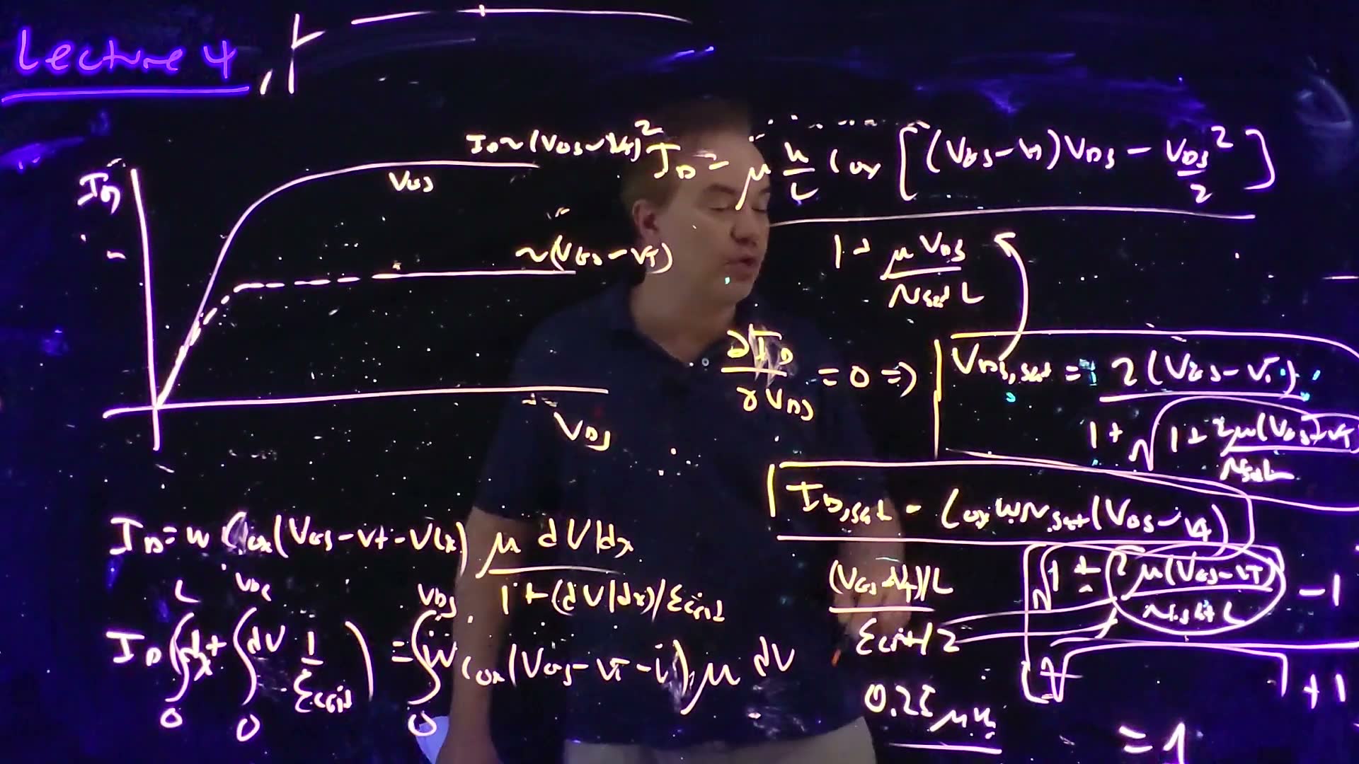
Earlier and lower (33:39–35:25). For the same $V_{GS}$VGS​, the velocity-saturated curve turns over at a smaller $V_{DSAT}$ and saturates at a smaller $I_{DSAT}$ than the long-channel model predicts.

Compare the two models below. Switch between them, shorten the channel, and watch the saturation points.

Model:Long-channelVelocity-saturatedBoth

channel length L

0.25 µm

threshold V_T

0.50 V

at V_GS = V_DD = 2.5 V: overdrive

2.00 V

(V_GS − V_T)/L vs ℰ_crit/2

80.0 vs 12.5 kV/cm (×6.40)

V_DSAT: long / vel.-sat.

2.00 / 1.08 V

I_DSAT long-channel

2046 µA

I_DSAT velocity-saturated

591 µA (29% of long)

limit C_oxWv_sat(V_GS − V_T)

1279 µA (46% reached)

Curves for V_GS = 1, 1.5, 2 and 2.5 V (those above V_T), labelled at the right. Dots mark V_DSAT; the dotted grey curve is the V_DSAT locus as V_GS sweeps up to 2.5 V. Both models are flat past V_DSAT: no DIBL or channel-length modulation here (Section 12). Device: W = 1 µm, t_ox = 5.4 nm, μ = 400 cm²/V·s, v_sat = 10⁷ cm/s, so ℰ_crit = 25 kV/cm.

What to notice.

• At $L = 10\,\mu\mathrm{m}$ the two families nearly coincide. The field $(V_{GS} - V_T)/L$ is well below $\mathcal{E}_{crit}/2$Ecrit​/2.
• At $L = 0.25\,\mu\mathrm{m}$ the velocity-saturated curves are far lower, their dots (at $V_{DSAT}$VDSAT​) sit far to the left, and their tops are almost evenly spaced: current linear in the overdrive. The long-channel tops spread out as a square.
• The readout “% reached” shows how close $I_{DSAT}$ is to the limit $C_{ox}Wv_{sat}(V_{GS} - V_T)$VT​). It approaches 100% only slowly as $L$ shrinks.

Worked example. added Both lengths at $V_{GS} = 2.5\,\mathrm{V}$2.5V, overdrive $U = 2\,\mathrm{V}$2V.

1. $L = 10\,\mu\mathrm{m}$10μm: $2\mu U/(v_{sat}L) = 2(400)(2)/(10^7 \times 10^{-3}) = 0.16$0.16, so $s = \sqrt{1.16} = 1.077$1.077.
2. $V_{DSAT} = 4/2.077 = 1.93\,\mathrm{V}$ (long-channel: 2 V). $I_{DSAT} = 6.39\times10^{-7} \times 10^{-4} \times 10^7 \times 2 \times (0.077/2.077) = 1.28\,\mathrm{mA} \times 0.0371 = 47.4\,\mu\mathrm{A}$47.4μA, 7% below the long-channel 51.2 µA.
3. $L = 0.25\,\mu\mathrm{m}$0.25μm: $2\mu U/(v_{sat}L) = 1600/(10^7 \times 2.5\times10^{-5}) = 6.4$6.4, so $s = \sqrt{7.4} = 2.720$2.720.
4. $V_{DSAT} = 4/3.720 = 1.08\,\mathrm{V}$1.08V, barely half the long-channel 2 V.
5. $I_{DSAT} = 1.28\,\mathrm{mA} \times (1.720/3.720) = 1.28 \times 0.462 = 0.591\,\mathrm{mA}$0.591mA.
6. The long-channel formula would say $\tfrac12 \times 2.56\times10^{-4} \times 4 \times 2^2 = 2.05\,\mathrm{mA}$ (now $W/L = 4$4), 3.5 times too much.
7. The limit $C_{ox}Wv_{sat}U = 1.28\,\mathrm{mA}$ is still twice the model’s $0.591\,\mathrm{mA}$0.591mA, although $(V_{GS} - V_T)/L = 80\,\mathrm{kV/cm}$ is 6.4 times $\mathcal{E}_{crit}/2 = 12.5\,\mathrm{kV/cm}$12.5kV/cm.

Common mistakes.

• Writing $2\mu(V_{GS} - V_T)/L$ under the root, as said at 29:46. Check units: the term must be dimensionless, so it needs $v_{sat}L$vsat​L.
• Using $C_{ox}Wv_{sat}(V_{GS} - V_T)$ whenever the criterion looks “large”. $(s - 1)/(s + 1)$ approaches 1 slowly: at 6.4× the critical field it is still only 0.46. Use the full formula when you can.
• Confusing current saturation (the flat part of every I–V curve, from pinch-off) with velocity saturation (carriers at $v_{sat}$vsat​). Long-channel devices show the first without the second.

Check yourself In a fully velocity-saturated device, V_GS − V_T doubles. What happens to I_DSAT? And if L is halved instead?

$I_{DSAT} = C_{ox}Wv_{sat}(V_{GS} - V_T)$ doubles with the overdrive (not 4× as in the long-channel model). It doesn’t depend on $L$ at all, so halving $L$ changes nothing in this limit. In the long-channel model, halving $L$ doubles the current.

8. Measuring the threshold voltage

The idea. The physics definition of $V_T$ (band bending) can’t be measured on a finished transistor. In practice $V_T$ is extracted from I–V measurements, and the answer depends on how.

Hand someone a transistor and they can measure only its terminal currents and voltages, not its band bending, so the physics definition is “completely useless” for that (36:17). There are several practical definitions, and you always have to ask which one was used (36:44).

Lecture04 @ 41:38Three definitions of V_T: physics, linear extrapolation (V_T,lin) and a current criterion at V_DS = V_DD (V_T,sat).

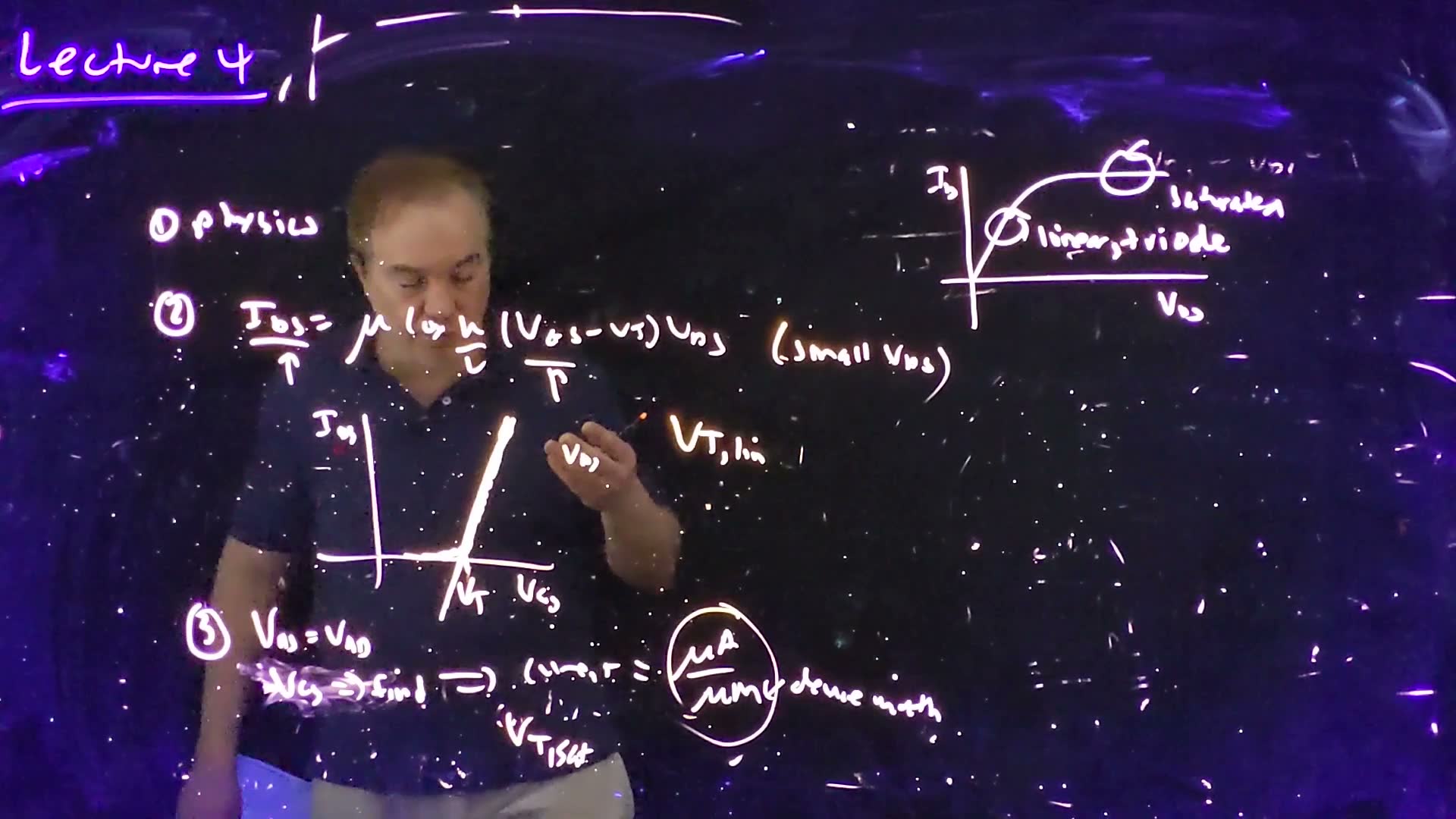
1. Physics (37:13): the band-bending definition of Chapter 3.

2. Linear extrapolation, $V_{T,lin}$ (38:19–39:54). Apply a small $V_{DS}$VDS​, say 100 mV. For small $V_{DS}$VDS​, velocity-saturated or not, the triode current is

   $$I_{DS} = \mu C_{ox}\frac{W}{L}(V_{GS} - V_T)\,V_{DS} ,$$

   a straight line in $V_{GS}$ that crosses the axis at $V_T$VT​. Plot $I_{DS}$ against $V_{GS}$VGS​. The real curve bends near the bottom, so fit the strongly linear part and extrapolate it to the axis.

3. Current criterion, $V_{T,sat}$ (39:54–41:22). Set $V_{DS} = V_{DD}$ and find the $V_{GS}$ at which the current reaches a chosen value per unit width, so many µA per µm. That $V_{GS}$ is called $V_T$VT​. It is very common, but the current level is not standard, so you need to know which one was used.

“Buyer beware”: one engineer’s $V_T$ is not another’s (41:51).

Worked example: the extrapolation is off by half of V_DS. added The Fall 2026 class added this. With the full triode formula, $I_D = \mu C_{ox}\frac{W}{L}V_{DS}\bigl(V_{GS} - V_T - V_{DS}/2\bigr)$VDS​/2), which is still a straight line in $V_{GS}$ but crosses the axis at $V_T + V_{DS}/2$VDS​/2.

1. At $V_{DS} = 50\,\mathrm{mV}$ the intercept is $V_T + 25\,\mathrm{mV}$25mV.
2. At the lecture’s 100 mV, it is $V_T + 50\,\mathrm{mV}$50mV. Subtract $V_{DS}/2$ from the intercept, or keep $V_{DS}$ small.

Check yourself Two vendors quote V_T = 0.40 V and 0.45 V for what may be the same transistor. What do you ask?

How each was defined: linear extrapolation (at what $V_{DS}$VDS​?) or a current criterion at $V_{DS} = V_{DD}$ (at what current per µm of width?). Different methods give different numbers for the same device.

9. PMOS, and the sign of the threshold

The idea. Every NMOS equation works for PMOS if you flip the voltage order and the current direction. The threshold, by convention, keeps the NMOS definition, so a PMOS threshold is negative.

Lecture04 @ 45:16PMOS substitutions (right), and 'enhancement mode' (centre top).

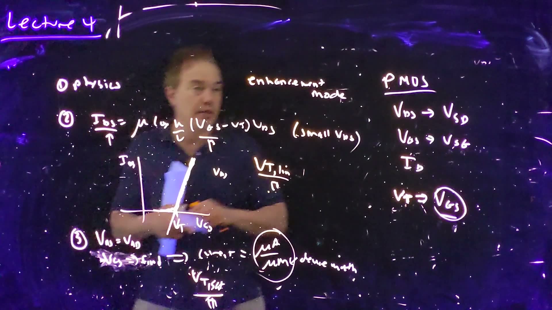
For PMOS (42:27–43:24):

• replace $V_{DS}$ with $V_{SD}$VSD​, and $V_{GS}$ with $V_{SG}$VSG​;
• the drain current flows out of the drain, the opposite direction.

With those swaps, every equation in this chapter still applies; the homework practises it.

Enhancement mode (43:35). All the transistors in this course are enhancement-mode devices: at $V_{GS} = 0$ there is no inversion layer and the device is off. A gate bias has to enhance it to turn it on.

The sign of $V_T$ (44:02–44:32). The threshold voltage is always defined as a value of $V_{GS}$VGS​, even for PMOS, where $V_{SG}$ would be more natural. So:

• an enhancement-mode NMOS has a positive $V_T$VT​, say 0.5 V;
• an enhancement-mode PMOS has a negative $V_T$VT​, say −0.5 V: it turns on when $V_{SG}$ exceeds 0.5 V.

People often drop the sign and say the PMOS threshold is “half a volt”. Everyone understands, but strictly it is −0.5 V.

Worked example. added A long-channel PMOS with $V_T = -0.5\,\mathrm{V}$−0.5V, source at 2.5 V, gate at 0.5 V, drain at 1.0 V.

1. $V_{SG} = 2.5 - 0.5 = 2.0\,\mathrm{V}$ and $V_{SD} = 2.5 - 1.0 = 1.5\,\mathrm{V}$1.5V.
2. The overdrive is $V_{SG} - |V_T| = 2.0 - 0.5 = 1.5\,\mathrm{V}$1.5V.
3. $V_{SD} = 1.5\,\mathrm{V} \ge 1.5\,\mathrm{V}$1.5V: the device is (just) saturated, and $I_D = \frac{\mu_p C_{ox}}{2}\frac{W}{L}(1.5)^2$2μp​Cox​​LW​(1.5)2, flowing out of the drain.

Check yourself A PMOS has V_T = −0.4 V. Its source is at 1 V. Is it on with the gate at 0.8 V? At 0.3 V?

$V_{SG} = 0.2\,\mathrm{V}$ at a gate of 0.8 V: below 0.4 V, so it is off. At a gate of 0.3 V, $V_{SG} = 0.7\,\mathrm{V}$0.7V: on, with 0.3 V of overdrive.

10. Dennard scaling

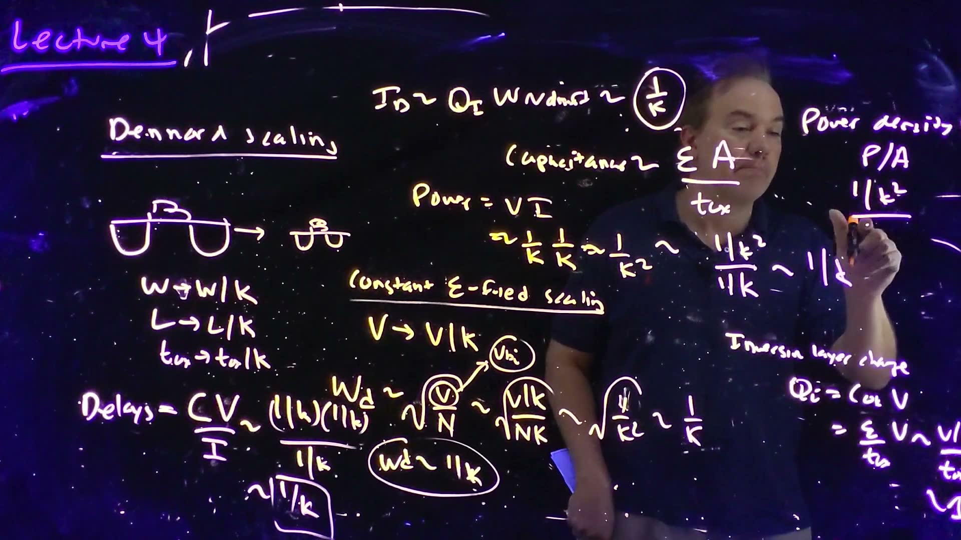
The idea. Shrink every dimension and every voltage by the same factor κ. The fields stay the same, and the transistor gets faster and lower-power while the power per area stays constant.

Moore’s law was about density: smaller transistors, more of them per chip, cheaper each (45:28). Bob Dennard of IBM showed that smaller transistors are also better: faster. That is Dennard scaling, the driver of decades of performance gains (45:49). The lecturer knew him at IBM, and mentions his other famous invention, the one-transistor DRAM cell (46:32–47:00).

The lecture says the paper appeared “in the late 1970s”. added It is Dennard and co-authors’ 1974 paper in the IEEE Journal of Solid-State Circuits.

Lecture04 @ 53:20Constant-field scaling, quantity by quantity. The right edge (Q_i and power density) is completed at 62:46.

The rules

Shrink by a factor $\kappa > 1$ (47:19–48:35):

• dimensions: $W \to W/\kappa$W/κ, $L \to L/\kappa$L/κ, $t_{ox} \to t_{ox}/\kappa$tox​/κ;
• voltages: $V \to V/\kappa$V/κ. Voltages and lengths shrink together, so fields stay constant. This is constant-field scaling. Higher fields would stress the devices and make them unreliable;
• doping: $N \to \kappa N$κN, so that depletion widths shrink too (next).

Quantity by quantity

What each quantity does under constant-field scaling (board, 48:38–53:40)

1. Depletion widths board: $W_d \sim \sqrt{V/N} \to \sqrt{(V/\kappa)/(\kappa N)} = W_d/\kappa$Wd​/κ. They shrink with everything else, but only if the doping rises by κ, and only if the whole voltage scales, including $V_{bi}$Vbi​. It doesn’t; hold that thought (49:35).
2. Capacitance board: $C \sim \varepsilon A/t_{ox} \sim (1/\kappa^2)/(1/\kappa) = 1/\kappa$1/κ. This is a device’s total capacitance, area times $C_{ox}$Cox​.
3. Inversion charge per area board: $Q_i = C_{ox}V = (\varepsilon/t_{ox})V \sim (1/\kappa)/(1/\kappa) = 1$1. Unchanged.
4. Current board: $I_D \sim Q_i W v_{drift} \sim 1 \cdot (1/\kappa) \cdot 1 = 1/\kappa$1/κ. The drift velocity is unchanged because the field is.
5. Delay board: charging a capacitance to a voltage with a current takes $CV/I \sim (1/\kappa)(1/\kappa)/(1/\kappa) = 1/\kappa$1/κ. Faster.
6. Power per transistor board: $P = VI \sim (1/\kappa)(1/\kappa) = 1/\kappa^2$1/κ2.
7. Power density board: $P/A \sim (1/\kappa^2)/(1/\kappa^2) = 1$1. Unchanged.

So each generation gives faster transistors, more of them, and the chip’s power per area doesn’t change. “This would be absolutely fantastic if it were true. Unfortunately, it’s not” (53:40).

Constant-field (Dennard) scaling by κboard

Quantity	Scales as
$W$W, $L$L, $t_{ox}$tox​, $V$V, $W_d$	$1/\kappa$
doping $N$	$\kappa$
capacitance $C$C, current $I$I, delay $CV/I$	$1/\kappa$
charge per area $Q_i$Qi​, field $\mathcal{E}$	1
power $VI$VI, area	$1/\kappa^2$
power density $P/A$	1

Holds when: all dimensions and all voltages (including V_bi and V_T) scale by 1/κ; doping by κ

Worked example. added One generation with $\kappa = 1.4$1.4, from the 0.25 µm node with a 2.5 V supply.

1. $L$L: $0.25/1.4 = 0.18\,\mu\mathrm{m}$0.18μm. Supply: $2.5/1.4 = 1.8\,\mathrm{V}$1.8V. These are the real next node and its supply.
2. Delay: $\times 1/1.4 = 0.71$0.71, so about 40% faster ($1.4\times$1.4× the frequency).
3. Power per transistor: $\times 1/1.4^2 = 0.51$0.51. Transistors per area: $\times 1.96$×1.96.
4. Power per area: $0.51 \times 1.96 = 1.0$1.0. Twice the transistors, 1.4 times faster, same heat per mm².

Check yourself Under constant-field scaling, why does the inversion charge per area not change, although the voltage falls?

$Q_i = C_{ox}V$ and $C_{ox} = \varepsilon/t_{ox}$ε/tox​. The voltage falls by κ, but $t_{ox}$ falls by κ too, so $C_{ox}$ rises by κ. The two cancel.

11. Why Dennard scaling broke: the subthreshold slope

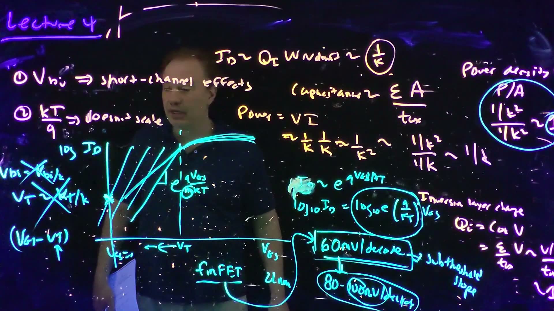
The idea. Two voltages refuse to scale: the built-in voltage and the thermal voltage $kT/q$kT/q. Because of $kT/q$kT/q, a transistor below threshold is never fully off, and its leakage grows tenfold for every 60 mV (at best) that the threshold is lowered. So $V_T$ can’t scale, and neither can the supply.

Lecture04 @ 62:46Why Dennard scaling broke: V_bi and kT/q don't scale; the subthreshold slope; FinFETs.

The two problems (54:18–55:19):

1. $V_{bi}$ doesn’t scale. It is fixed by the band gap (Chapter 3). So depletion widths don’t shrink as they should, which leads to short-channel effects (Section 12).
2. $kT/q$ doesn’t scale. It is set by the temperature.

Subthreshold current

So far a transistor has been on above $V_T$ and off below. Really, it doesn’t switch off to zero (55:41). Plot $\log I_D$ against $V_{GS}$ (56:15): above threshold you see the normal characteristic; below threshold the current falls exponentially as the gate voltage drops (56:45):

$$I_D \sim e^{qV_{GS}/kT} .$$

The reason: what turns the device off is a barrier in the MOS structure that carriers must get over. The gate lowers that barrier, and the number of carriers with enough thermal energy to cross it grows exponentially (56:45–57:16). Chapter 2’s $e^{-E/kT}$ tails are at work again.

Sixty millivolts per decade (board, 57:37–58:23)

1. Take $\log_{10}$ of $I_D \propto e^{qV_{GS}/kT}$ board: $\log_{10}I_D = \log_{10}e\cdot\dfrac{q}{kT}V_{GS} + \text{const}$const.
2. So $\log_{10}I_D$ is a straight line in $V_{GS}$ with slope $\log_{10}e \cdot q/kT$ decades per volt.
3. Invert it added: the gate voltage per decade of current is $\dfrac{kT/q}{\log_{10}e} = \dfrac{kT}{q}\ln 10$qkT​ln10.
4. At room temperature, $0.02585 \times 2.303 = 0.0595\,\mathrm{V}$0.0595V: about 60 mV per decade board. This is the subthreshold slope.

To change the drain current by 10×, you must change the gate voltage by 60 mV (58:35).

Why V_T can’t scale

Dennard scaling also assumed $V_T$ scales by κ (59:08). Lower the threshold and the whole curve slides left, but its slope can’t change. At $V_{GS} = 0$0, where the device is supposed to be off, the current rises: more and more leakage (59:35–60:03).

Real devices are worse: the factor m

60 mV/decade is the ideal, best case. Gate control over the barrier is not perfect, so most devices follow (60:03–60:32)

$$I_D \sim e^{qV_{GS}/mkT}$$

so the subthreshold slope becomes $m\,\frac{kT}{q}\ln 10$mqkT​ln10, with $m > 1$1: typically 80, even 100 mV/decade. $m$ reflects how good the device’s electrostatics are, and scaling made them worse. At the 22 nm node, bulk CMOS reached about 100 mV/decade, which “was just intolerable” (61:16).

For 14/16 nm the industry switched to FinFETs, whose gate wraps around the channel. Better electrostatics brought the slope back near 60 mV/decade. That, more than anything, is what FinFETs are for (61:16–61:55). added Intel’s 22 nm process was already a FinFET one (the board notes “finFET, 22 nm”); the foundries switched at 14/16 nm.

Subthreshold slopeboard

$$I_D \sim e^{qV_{GS}/mkT}$$$$S = m\,\frac{kT}{q}\ln 10 \approx m \times 60\ \mathrm{mV/decade}$$

The board writes the 60 mV/decade and the 80–100 mV/decade; $S$ and the $\ln 10$ form are added. The 60 mV limit belongs to carriers crossing a barrier thermally, as in a MOSFET added.

Holds when: below threshold; ideal m = 1 gives the best case; room temperature for the 60 mV figure

threshold V_T

0.40 V

ideality factor m

1.00

subthreshold slope m(kT/q) ln 10

59.5 mV/decade

decades from V_T down to 0 V

6.7

leakage at V_GS = 0

4.0×10⁻¹⁴ A/µm

compared with the grey curve

the same

I_on/I_off at V_GS = 1.2 V

1.3×10⁹

Below V_T the current falls by 10× for every 60 mV of gate voltage: a straight line on this log scale. Lowering V_T slides the whole curve left, and the line then crosses V_GS = 0 at a higher current. The curve is pinned to 100 nA/µm at V_T; above threshold it is only a smooth sketch (not from the lecture), so read the slope and the leakage, not the on-current.

What to notice.

• Drag $V_T$ down: the blue curve slides left, and the leakage at $V_{GS} = 0$ jumps tenfold for every $S$ volts.
• Raise $m$m: the line below threshold tilts flatter, so the same $V_T$ leaves far more leakage at 0 V.
• To keep leakage at the grey curve’s level with $m = 1.5$1.5, $V_T$ must rise, not fall.

The net result (61:55–62:54). With $V_{bi}$ and $kT/q$ fixed, $V_T$ can’t scale. To keep performance the overdrive $V_{GS} - V_T$ must be kept, so the supply can’t scale either. Then power density no longer stays constant: it rises, steeply. Managing power has become one of the biggest problems in chip design.

Worked example. added A threshold of 0.3 V.

1. At 60 mV/decade, from $V_{GS} = V_T$ down to 0 the current falls $0.3/0.06 = 5$ decades: $10^5$×.
2. Lower $V_T$ by 120 mV, two decades’ worth: the leakage at $V_{GS} = 0$ rises $10^2 = 100$×. (With the exact 59.5 mV, $10^{0.12/0.0595} = 104$×.)
3. With $m = 1.5$ ($S = 89\,\mathrm{mV/decade}$S=89mV/decade), the same 0.3 V gives only $0.3/0.089 = 3.4$ decades of turn-off.

Common mistakes.

• Treating “60 mV per decade” as a slope you can improve with better process alone. For a MOSFET at room temperature it is the floor; real devices are worse ($m > 1$m>1).
• Reading the slope backwards. A smaller mV/decade is better: less gate voltage per decade of current.

Check yourself A device has S = 100 mV/decade and V_T = 0.4 V. By how many decades is its current at V_GS = 0 below its current at V_T? What would S = 60 mV/decade give?

$0.4/0.1 = 4$ decades ($10^4$104×). At 60 mV/decade, $0.4/0.06 = 6.7$ decades: about 500 times less leakage for the same threshold.

Check yourself An NFET carries 10 µA/µm at V_GS = V_T = 200 mV, and its subthreshold slope is 90 mV/decade. How much does it leak per µm of width at V_GS = 0?

From $V_T$ down to 0 is $200/90 = 2.22$ decades, a factor of $10^{2.22} = 167$167. So the leakage is $10\,\mu\mathrm{A}/167 \approx 60\,\mathrm{nA}/\mu\mathrm{m}$60nA/μm. A PFET with the same numbers ($-200$−200 mV) leaks the same. In a static inverter only the device that is off leaks, with the full $V_{DD}$ across it; Chapter 6 turns this current into leakage energy. The MT23 key prints 60 pA/µm, but the arithmetic gives nA. (This is MT23-1b and MT24-2b.)

Check yourself An NFET carries I_D = 10 µA at V_GS = V_T = 1 V, with a subthreshold slope of 60 mV/decade at 300 K. What is I_D at V_GS = 0 at 300 K? And at 400 K?

At 300 K: $1000/60 = 16.7$ decades, so $I_D = 10\,\mu\mathrm{A} \times 10^{-16.7} = 2.15\times10^{-22}\,\mathrm{A}$10−22A.

At 400 K added: the slope is $m\,(kT/q)\ln 10$m(kT/q)ln10, proportional to the absolute temperature, so it becomes $60 \times 400/300 = 80\,\mathrm{mV/decade}$80mV/decade. Then $1000/80 = 12.5$ decades, and $I_D = 10\,\mu\mathrm{A} \times 10^{-12.5} = 3.16\times10^{-18}\,\mathrm{A}$10−18A, about 15 000 times more. The lecture says only that $kT/q$ “is set by the temperature” (55:19); this scaling is the added step. Like the exam, the answer holds $V_T$ and the 10 µA at $V_T$ fixed. (This is MT17-1c.)

12. Short-channel effects: DIBL and threshold roll-off

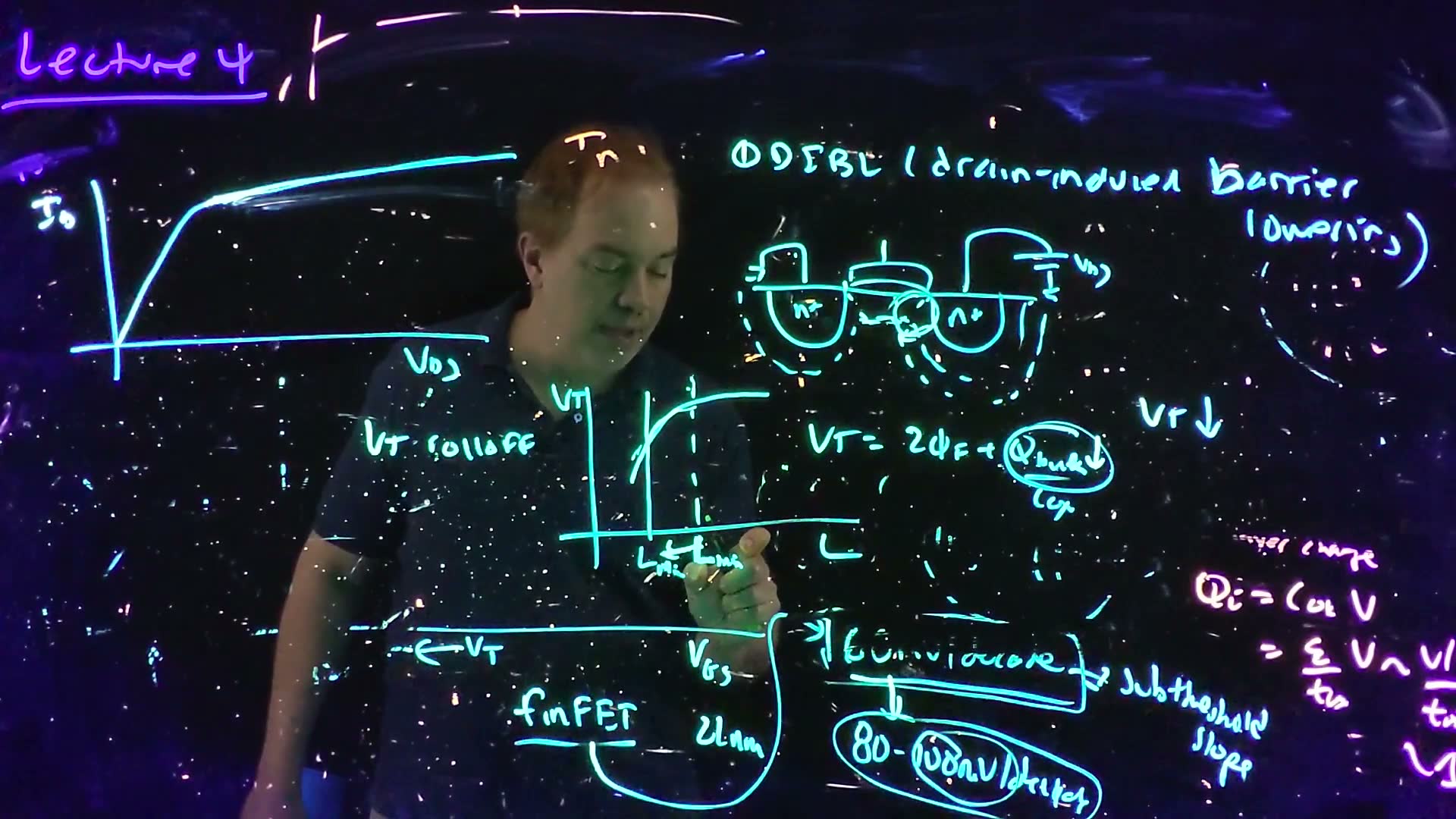
The idea. In a short transistor the source and drain depletion regions reach under the gate and take over part of the depletion charge the gate is supposed to control. The threshold then drops, with more drain voltage (DIBL) and with shorter channels (roll-off).

Lecture04 @ 68:40DIBL (top right), its effect on the I–V (top left), and V_T roll-off (centre).

The short-channel effects all have a similar cause (63:24). They follow from the depletion widths that wouldn’t scale (Section 11).

DIBL: drain-induced barrier lowering

Look at the depletion regions (64:02–65:24):

• under the gate there is the depletion region from Chapter 3, holding the charge $Q_{bulk}$Qbulk​;
• around the source and the drain there are junction depletion regions;
• raising $V_{DS}$ reverse-biases the drain junction harder, so the drain’s depletion region grows (Chapter 3). Since depletion widths no longer scale, it reaches under the gate.

Some of the depletion charge under the gate now belongs to the drain. Recall $V_T = V_{FB} + 2\phi_F + Q_{bulk}/C_{ox}$Qbulk​/Cox​: the gate has to support less $Q_{bulk}$Qbulk​, so $V_T$ falls as $V_{DS}$ rises (65:24). That is DIBL.

What it does to the I–V (66:03–66:42). In saturation, raising $V_{DS}$ should leave the current flat. With DIBL, more $V_{DS}$ means a lower $V_T$VT​, a larger overdrive and more current: the saturated curve slopes upward. The device has a finite output conductance and no longer looks like a current source.

Threshold roll-off

Plot $V_T$ against channel length (67:15). As $L$ shrinks, the source and drain depletion regions (mostly the drain’s, being reverse-biased) control a larger share of the charge under the gate, and $V_T$ drops: $V_T$ roll-off.

Why care? Lithography can’t print $L$ exactly. If the minimum length sits where the curve is steep, every small error in $L$ becomes a large error in $V_T$VT​. So choose $L_{min}$ where $V_T(L)$ is as flat as possible (68:13).

With some doping tricks, $V_T$ first rises slightly as $L$ shrinks and then rolls off. This is inverse roll-off; the same argument about where to put $L_{min}$ applies (68:45).

Check yourself A process has a steep V_T roll-off at its minimum length. Why is that a problem even if the average V_T is on target?

Every transistor’s $L$ varies a little from lithography. On a steep part of the $V_T(L)$ curve, those small length variations become large threshold variations from device to device.

13. Gate leakage

The idea. Oxides thinned with scaling eventually get thin enough for electrons to tunnel straight through them. The gate then leaks, and the leakage grows about tenfold for every 2 Å of thinning.

Lecture04 @ 72:49Gate leakage from 0.25 µm to 90 nm (left); inverse roll-off (centre).

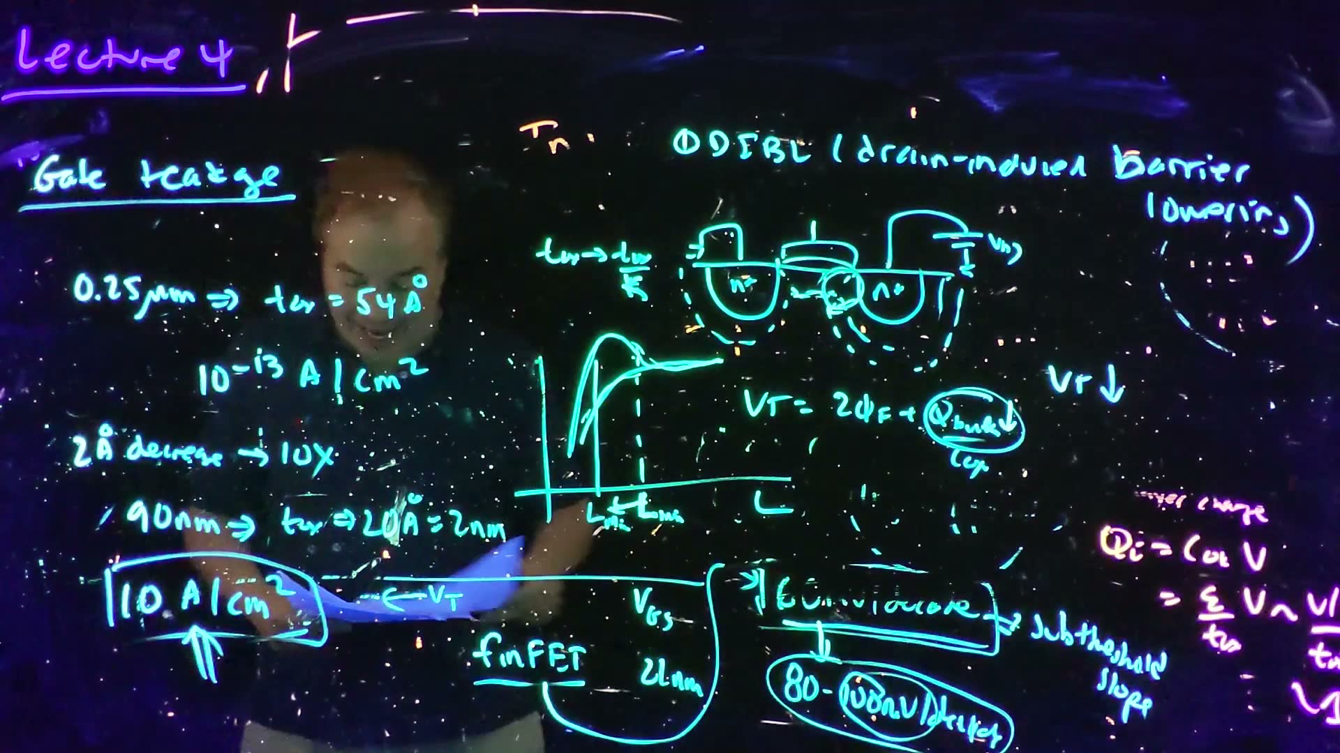
The gate should be a perfect insulator: no gate current (69:35). But Dennard scaling thins the oxide by κ every generation, and eventually electrons tunnel quantum-mechanically through it: a gate leakage current (70:02).

The lecture’s numbers (70:39–71:51):

• at the 0.25 µm generation, $t_{ox} = 54\,\text{Å} = 5.4\,\mathrm{nm}$ and the gate current is about $10^{-13}\,\mathrm{A/cm^2}$10−13A/cm2: effectively zero;
• every 2 Å thinner gives about 10× more current;
• at 90 nm, $t_{ox} \approx 20\,\text{Å} = 2\,\mathrm{nm}$ (the lecturer first says “two angstroms” and corrects himself), and the leakage is about $10\,\mathrm{A/cm^2}$10A/cm2.

About 10 A/cm² is usually treated as the upper limit, and technologies don’t let gate leakage go past it. Beyond 90 nm the oxide couldn’t be thinned further, so the industry switched to high-κ dielectrics (72:19): a physically thicker layer of a material with a higher dielectric constant gives the same $C_{ox}$Cox​, so it acts like a thinner oxide while keeping the leakage down.

Checking the numbers. added The two end points span $\log_{10}(10/10^{-13}) = 14$ decades over $54 - 20 = 34\,\text{Å}$34A˚: about 2.4 Å per decade. At exactly 2 Å per decade the same thinning would give 17 decades, $10^4\,\mathrm{A/cm^2}$104A/cm2. So read “10× per 2 Å” as a rule of thumb (2–2.5 Å per decade), and the end points as the lecture’s data.

Check yourself An oxide leaks 1 A/cm². Using 10× per 2 Å, how much thinner can it get before reaching the 10 A/cm² limit? What κ_ox would let a 4 nm layer have the C_ox of 2 nm of SiO₂?

One decade: about 2 Å. For equal $C_{ox} = \kappa\varepsilon_0/t$κε0​/t, the thicker layer needs twice the dielectric constant: $\kappa = 2 \times 3.9 = 7.8$7.8.

Formulas to remember

Formula	Meaning
$v_{drift} = \mu\mathcal{E}$μE; $\mu$ in cm²/V·s	low-field drift
$v_{sat} \sim 10^7$ (electrons), $5\times10^6$ (holes) cm/s	saturation velocities
$I_D = W Q_i(x) v_{drift}$WQi​(x)vdrift​, $Q_i(x) = C_{ox}(V_{GS} - V_T - V(x))$	current = charge × velocity
$I_D = \mu C_{ox}\frac{W}{L}\bigl[(V_{GS} - V_T)V_{DS} - V_{DS}^2/2\bigr]$	long-channel triode
$V_{DSAT} = V_{GS} - V_T$VT​, $I_{DSAT} = \frac{\mu C_{ox}}{2}\frac{W}{L}(V_{GS} - V_T)^2$	long-channel saturation (square law)
$v_{drift} = \dfrac{\mu\mathcal{E}}{1 + \mathcal{E}/\mathcal{E}_{crit}}$1+E/Ecrit​μE​, $v_{sat} = \mu\mathcal{E}_{crit}$	velocity-saturation fit, $\mathcal{E}_{crit} \sim 10^4$ V/cm
$I_D = I_{D,\text{long}}/(1 + \mu V_{DS}/v_{sat}L)$	velocity-saturated triode
$V_{DSAT} = \dfrac{2(V_{GS} - V_T)}{1 + s}$1+s2(VGS​−VT​)​, $I_{DSAT} = C_{ox}Wv_{sat}(V_{GS} - V_T)\dfrac{s - 1}{s + 1}$	velocity-saturated; $s$ as in Section 7
$I_{DSAT} = C_{ox}Wv_{sat}(V_{GS} - V_T)$	short channels: field $\gg \mathcal{E}_{crit}/2$
PMOS: $V_{DS} \to V_{SD}$VSD​, $V_{GS} \to V_{SG}$VSG​; $V_T < 0$	signs
$W, L, t_{ox}, V \to /\kappa$/κ, $N \to \kappa N$κN: delay $1/\kappa$1/κ, power $1/\kappa^2$1/κ2, $P/A$ 1	constant-field scaling
$S = m\frac{kT}{q}\ln 10 \ge 60$ mV/decade	subthreshold slope

The lecture’s boards

Lecture04 @ 05:29 drift velocity, mobility, v_sat

Lecture04 @ 13:21 I_D = W Q_i v_drift and the integral

Lecture04 @ 20:48 parabola, pinch-off, saturation

Lecture04 @ 22:48 why the square: Q_i and v_drift

Lecture04 @ 33:04 velocity-saturated I_D, V_DS,sat, I_D,sat

Lecture04 @ 35:05 long-channel vs velocity-saturated I–V

Lecture04 @ 41:38 threshold definitions: V_T,lin, V_T,sat

Lecture04 @ 45:16 PMOS substitutions, enhancement mode

Lecture04 @ 53:20 Dennard (constant-field) scaling

Lecture04 @ 62:46 why it broke: subthreshold slope, FinFET

Lecture04 @ 68:40 DIBL and V_T roll-off

Lecture04 @ 72:49 gate leakage; inverse roll-off