23. Test signatures, electromigration, clocks and energy

Lecture 22 is, in the lecturer’s own word, a “grab bag”: four topics that finish the course’s circuit material before the last lecture turns to devices. It opens by finishing built-in self-test: a few flip-flops and one XOR gate, a linear feedback shift register, make a long pseudo-random test pattern, and a second such register folds the circuit’s whole response into a short signature. Then electromigration: why a steady current slowly drags a wire’s metal along with it, why supply straps and vias are the wires at risk, and the current-density limits in mA/µm² that size them. The middle of the lecture is clock distribution: the four things a clock network is judged by (skew, jitter, power and latency), why a network with a short latency has less skew and jitter, and the three ways chips have distributed their clocks (grids, H-trees and tree-driven grids). The lecture ends with energy-constrained design: the two kinds of wasted power and the gating that removes each, the energy–delay curve, and the supply voltage as the knob that moves a design along it (DVFS).

Two sections at the end are added. The lecture stops at “you can operate below threshold”; two past final parts ask how far below. Section 15 finds the lowest supply at which a subthreshold inverter still gives a valid logic level, and Section 16 finds when a lower supply stops saving energy.

After this chapter you can:

1. build a maximum-length LFSR, list its states, and compress a response stream into a signature;
2. explain electromigration, say why supply lines and vias are at risk and why burn-in runs hot, and size a wire from a current-density limit;
3. define skew, jitter, power and latency, and explain why a clock network with low latency has less skew and jitter;
4. compare a grid, an H-tree and a tree-driven grid, and explain why tree delays are tuned wire for wire and silicon for silicon;
5. name the two sources of wasted power and the gating that removes each;
6. read an energy–delay curve, use $V_{DD}$ to move along it, and explain DVFS;
7. find the lowest supply at which a subthreshold inverter still gives a valid logic level, and decide whether a logic block has a minimum-energy supply above it.

Boxes and equations marked board were written in the lecture. Parts marked added are explanations or examples this guide adds. The lecture writes almost no equations (only $x^4 + x + 1$1, $2^n - 1$ and the current-density limits), so nearly every worked example here is added and uses illustrative values, built from the course’s earlier models.

Symbols

Symbol	Meaning	Unit	First appears
$n$	the number of flip-flops in an LFSR or signature register	—	§1
$Q_i$Qi​, $D_i$	the output and the input of flip-flop $i$	—	§1
$\oplus$	exclusive OR (XOR): 1 when its inputs differ	—	§1
$J$J, $J_{max}$	current density in a wire, $I/(wt)$I/(wt); its allowed limit	mA/µm²	§3, §4
$I$	a wire’s current (DC unless stated)	mA	§3
$w$w, $t$	a wire’s width and thickness	µm	§4
$t_L$	latency: the clock network’s delay from its root to a leaf flip-flop added	ps	§6
$\delta$	signed skew (Chapter 14): how much later the capturing flip-flop’s clock arrives	ps	§6
$t_{skew}$tskew​, $t_{jitter}$	the size of the static and of the transient spread in clock arrival	ps	§6
$S_V$	the supply sensitivity of delay, $(V_{DD}/t)(\partial t/\partial V_{DD})$(VDD​/t)(∂t/∂VDD​); Chapter 21 and FS1 write it $S$	—	§6
$V_{DD}$VDD​, $V_T$	supply voltage; threshold voltage	V, mV	§6
$D$D, $k$	the side of a square chip; the number of levels of an H-tree	mm	§8, §9
$p$	the pitch of a clock grid	mm	§8
$R$R, $\Delta C$	a driver’s resistance; a change of load capacitance	Ω, fF	§9
$C_{clk}$Cclk​, $f$	the clock network’s capacitance; the clock frequency	pF, GHz	§8, §12
$R_{on}$	the on-resistance of a power-gating switch	Ω	§12
$E$E, $E_{dyn}$Edyn​, $E_{leak}$	energy per operation: total, switching, leakage	J (or $10^{-3}$ V² per $N_gC$Ng​C)	§13, §16
$S$	the subthreshold slope: gate voltage per decade of current	mV/decade	§12, §15
$kT/q$	the thermal voltage, 26 mV at room temperature	mV	§15
$I_{off}$Ioff​, $I_{on}$	a transistor’s current at $V_{GS} = 0$ and at $V_{GS} = V_{DD}$	nA	§15
$V_{out}$Vout​, $V_{fn}$	an inverter’s output voltage; the lowest supply at which the low output is at most $0.1V_{DD}$ added	mV	§15
$N$N, $N_g$	gates on the critical path (logic depth); gates in the whole block added	—	§16
$\alpha$	the fraction of the block’s nodes that rise in one operation added	—	§16
$T$	the time one operation takes	ns	§16
$u$u, $K$	the supply in units of $S/\ln 10$S/ln10, $u = V_{DD}\ln 10/S$VDD​ln10/S; the block constant $K = N/(4\alpha)$ added	—	§16

1. LFSRs: pseudo-random test patterns

You need

Logic BIST (Chapter 22). A tester checks a die by shifting patterns into its scan chains, clocking the logic once, and shifting the responses out (the scan test of Chapter 22). Built-in self-test puts that job on the chip. LBIST (logic BIST) generates the patterns, runs them through the scan chains and checks the responses on chip; ABIST does the same for memory arrays.

LBIST and ABIST (Chapter 22, after the board at Lecture21 @ 61:01). This section builds the LFSR box; Section 2 builds SIG. Original figure ↗

A D flip-flop (Chapter 13) copies its input D to its output Q at each clock edge and holds it until the next. Flip-flops in a row, each Q wired to the next D, form a shift register: at every edge each bit moves one place along.

XOR added. $a \oplus b$ is 1 when $a$ and $b$ differ and 0 when they are equal. So $a \oplus 0 = a$a, $a \oplus 1 = \bar a$aˉ, and $a \oplus a = 0$0.

The question. LBIST needs a pattern generator on the chip: something small that produces a long, random-looking stream of bits to shift into the scan chains. How do four flip-flops and one XOR gate make such a stream, how long does it run before it repeats, and why is that length $2^n - 1$ and not $2^n$2n?

Where the two registers of this section and the next sit added, after the lecture (00:37–05:59). A pattern generator (PRBS, from an LFSR) feeds the scan chains of the circuit under test (CUT); the responses go into a signature register (SIG), whose final contents are compared (=) with the expected signature; a BIST controller sequences the run. The expected signature is drawn as the shaded register SIG₀; ✓ and ✗ mark pass and fail.

From a shift register to a pattern generator (board, 00:37–03:45)

1. What LBIST needs board. A pattern generator that makes a PRBS, a pseudo-random bit sequence: a stream that looks random but is fully determined, so a simulation of the good circuit can predict every response (00:51).
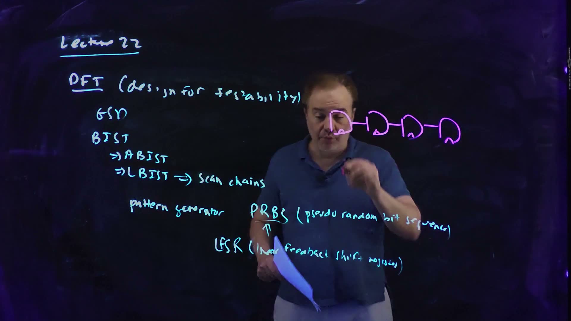
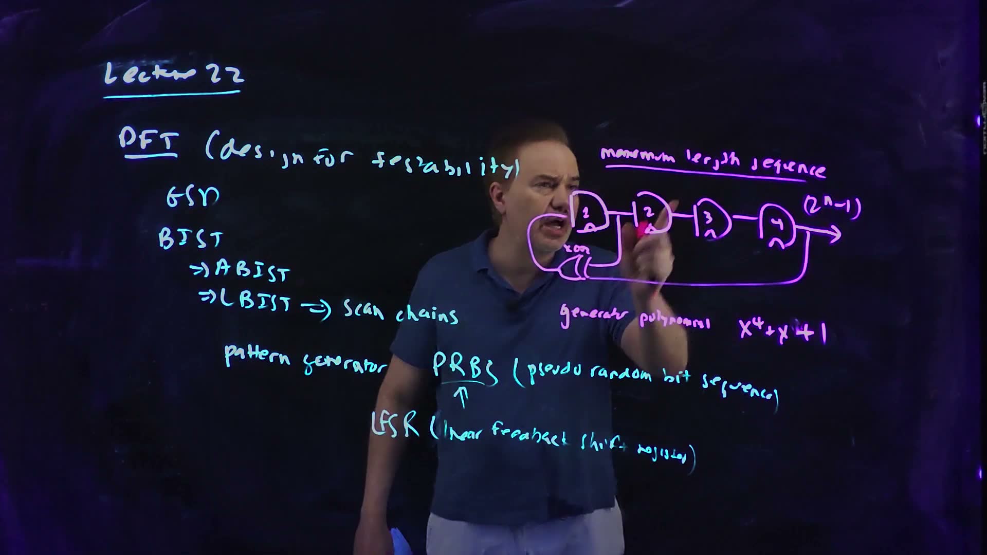
2. The circuit board (01:40–02:28). Four flip-flops in a ring, numbered 1 to 4. Each $Q_i$ drives $D_{i+1}$Di+1​, as in a shift register. Flop 1’s input comes from an XOR of $Q_1$ and $Q_4$Q4​: the outputs of flip-flops one and four, “feeding them round” to the input. That is the linear feedback shift register (LFSR). The output is taken from flop 4.
3. The rule, one clock at a time added. At each edge, $Q_1^{+} = Q_1 \oplus Q_4,\quad Q_2^{+} = Q_1,\quad Q_3^{+} = Q_2,\quad Q_4^{+} = Q_3 .$ The superscript + means “after the edge”. Everything moves one place right, and the new bit entering at the left is the XOR of the old first and last bits.
4. The name of the feedback board (02:28). The board names this feedback by its generator polynomial, $x^4 + x + 1$1. added Which end of the register counts as $x^0$ is a convention: read from the other end, the same register is $x^4 + x^3 + 1$1. The algebra is not needed here; what matters is the register drawn and the rule in step 3.
5. How long it runs board (03:05). “The longest I can run before I repeat myself is 2 to the n minus 1”: for $n = 4$ flip-flops, 15 clocks. Feedback that reaches that length gives a maximum-length sequence, and the board’s register is one.
6. Other uses (03:32). The same PRBS generators test communication links, where a receiver compares the received bits with its own copy to measure the bit error rate.

The board’s four-flop LFSR board, redrawn (Lecture22 @ 05:53; drawn 01:40–03:00). The XOR of $Q_1$ and $Q_4$ feeds $D_1$D1​; each $Q_i$ feeds $D_{i+1}$Di+1​; the output leaves flop 4. The board names the feedback $x^4 + x + 1$ and marks the output with the period $2^n - 1$1. The flip-flops are drawn as boxes with a clock input (the board draws D shapes).

The board (Lecture22 @ 05:53)

Lecture22 @ 05:53The LBIST pattern generator: a PRBS from a four-flop LFSR, x⁴ + x + 1, period 2ⁿ − 1; and the six-flop signature register below it.

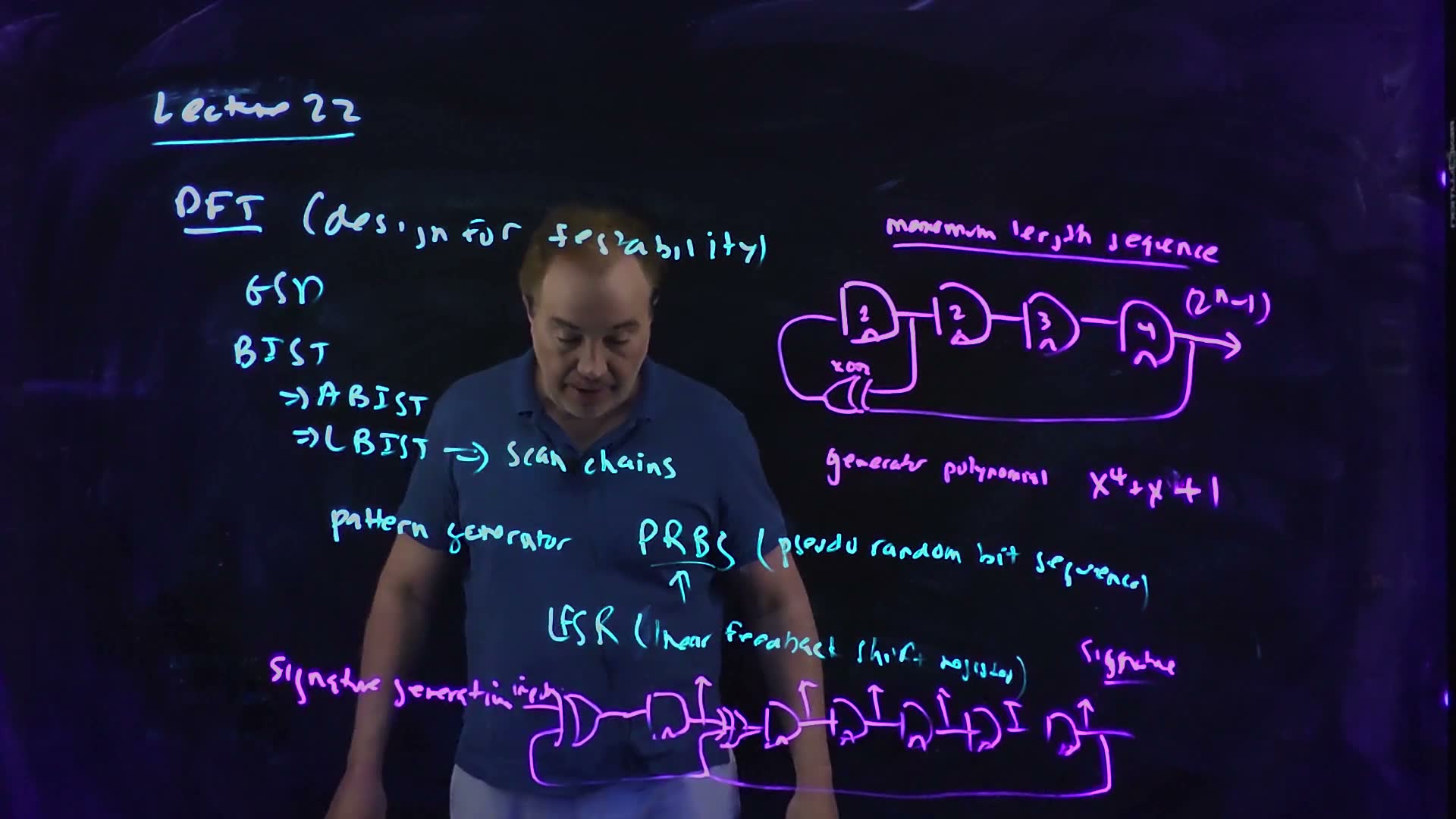
Fair copy of the board above (Lecture22 @ 05:53), mark for mark in its own layout, all in black. A cyan pen wrote the recap down to “LFSR (linear feedback shift register)”; a pink pen wrote the rest: the four-flop LFSR, “maximum length sequence”, the generator polynomial and the six-flop signature register. The pink pen carries the topic on rather than marking a layer over the cyan, so it takes no accent. Nothing is hidden: the lecturer stands behind the strokes (checked against 00:57 and 05:08). The flip-flops keep the board’s D shapes, and the LFSR’s XOR faces left, as drawn. The hand’s “GSD” (general scan design) ends in an open loop that reads like “n”. The words are set smaller than the hand, and “polynomial” and x⁴ + x + 1 sit a little right of their place to clear the wider type.

Walking the register through its states

A worked example: the board's LFSR from 0001 (added)

1. The seed. Load $Q_1Q_2Q_3Q_4 = 0001$0001. Any nonzero state would do (step 4 says why not zero).

2. The first clock. $Q_1^{+} = Q_1 \oplus Q_4 = 0 \oplus 1 = 1$1, and the other bits shift right: $1000$1000.

3. Keep going. Each column below is one clock later; the leftmost bit of each state is the XOR of the first and last bits of the state before it.

   Clock	0	1	2	3	4	5	6	7	8	9	10	11	12	13	14	15
   $Q_1Q_2Q_3Q_4$	0001	1000	1100	1110	1111	0111	1011	0101	1010	1101	0110	0011	1001	0100	0010	0001

   After 15 clocks the register is back at 0001, and from then on the sequence repeats.

4. Why 15, not 16. The 15 states are all different, and they are every 4-bit pattern except 0000. That one is excluded because it is a trap: $0 \oplus 0 = 0$0, so 0000 maps to itself forever. A register seeded with zeros produces only zeros. So the most an $n$-flop register can visit is the $2^n - 1$ nonzero states.

5. The output stream. Reading $Q_4$ over one period gives 100011110101100: 8 ones and 7 zeros, as balanced as an odd length allows. It never has more than three zeros in a row, because four zeros in a row would mean the state 0000.

6. Not every feedback is maximal. Move the tap from $Q_1$ to $Q_2$ ($Q_1^{+} = Q_2 \oplus Q_4$Q1+​=Q4​, the polynomial $x^4 + x^2 + 1$1): from 0001 the register returns after only 6 clocks. The other nine nonzero states form separate, shorter cycles. A pattern generator needs a feedback that is known to be maximal, and tables of such polynomials exist for every $n$n.

The period of a maximum-length LFSRboard

$$\text{period} = 2^n - 1$$

Holds when: n flip-flops with a maximal (primitive) feedback, such as the board's x⁴ + x + 1 for n = 4, and a nonzero seed; the all-zero state maps to itself and is never reached from a nonzero one

Memorize it, with its reason: $2^n$ states, minus the all-zero trap.

Traps.

• $2^n$ states. The all-zero state is excluded; an $n$-flop LFSR has period $2^n - 1$ at most.
• Seeding with zeros. A reset that clears every flip-flop leaves the generator stuck at 0000; the seed must be nonzero.
• Any taps will do. Only some feedbacks are maximal; the $Q_2$Q2​, $Q_4$ taps above give a period of 6.

Check yourself How many clocks does a 20-flop maximum-length LFSR run before it repeats?

$2^{20} - 1 =$ 1,048,575: about a million patterns from twenty flip-flops and a few XOR gates.

Check yourself Start the board's register at 1111. What are the next three states, and after how many clocks does 1111 come back?

Each new first bit is $Q_1 \oplus Q_4$ of the state before. From 1111: $1 \oplus 1 = 0$0, so 0111; then $0 \oplus 1 = 1$1: 1011; then $1 \oplus 1 = 0$0: 0101. The register is maximal, so every nonzero state lies on the same 15-state cycle (it is the walk above, entered at clock 4): 1111 returns after 15 clocks.

Check yourself Why can the output stream of an n-flop LFSR never contain n zeros in a row?

The output is $Q_n$Qn​, and each bit of the register reaches the output a few clocks later: $Q_3$ one clock later, $Q_2$ two, $Q_1$ three. So four zeros in a row out of $Q_4$ are the four bits the register held at one moment: all four flip-flops held 0. That is the trap state, which a nonzero seed never reaches.

2. Signature registers: compressing the response

You need

The LFSR (Section 1). Flip-flops in a shift register with an XOR feeding back from the outputs; with a maximal feedback, $n$ flip-flops cycle through all $2^n - 1$ nonzero states before repeating.

The board’s four-flop LFSR (Section 1). Original figure ↑

The response (Chapter 22). After each test pattern is captured, the scan chain shifts the logic’s response out of scan_out one bit per clock. A test of thousands of patterns gives millions of response bits, and each must match what a simulation of the good circuit predicts.

The question. Comparing millions of response bits one by one on chip would need the whole expected stream stored beside the circuit. How can a register of a few flip-flops fold the whole stream into a short signature that is compared once, and what can such a compression miss?

From an LFSR to a signature register (board, 04:02–05:59)

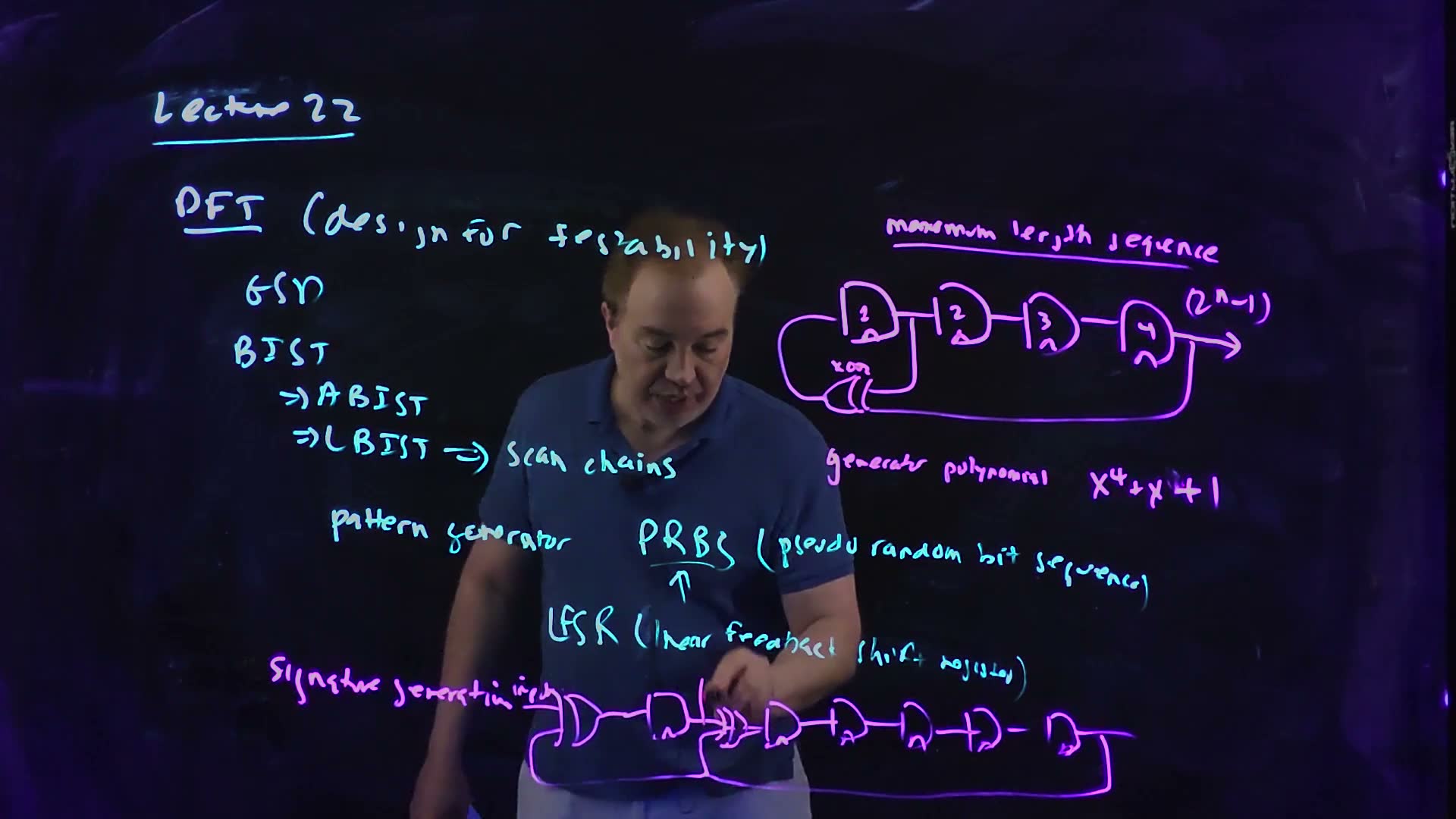
1. A second LFSR, with an input board (04:26–04:49). Six flip-flops in a row. The incoming response bits enter through an XOR in front of flop 1, together with $Q_6$Q6​; a second XOR in front of flop 2 combines $Q_1$ with $Q_6$Q6​; the rest simply shift. As equations added: $D_1 = \text{in} \oplus Q_6,\quad D_2 = Q_1 \oplus Q_6,\quad D_3 = Q_2,\ \ldots,\ D_6 = Q_5 .$
2. Clock the response in (05:17). Reset the register, then clock the entire response stream through it, one bit per clock. Every bit is mixed into the state, and the feedback keeps mixing it.
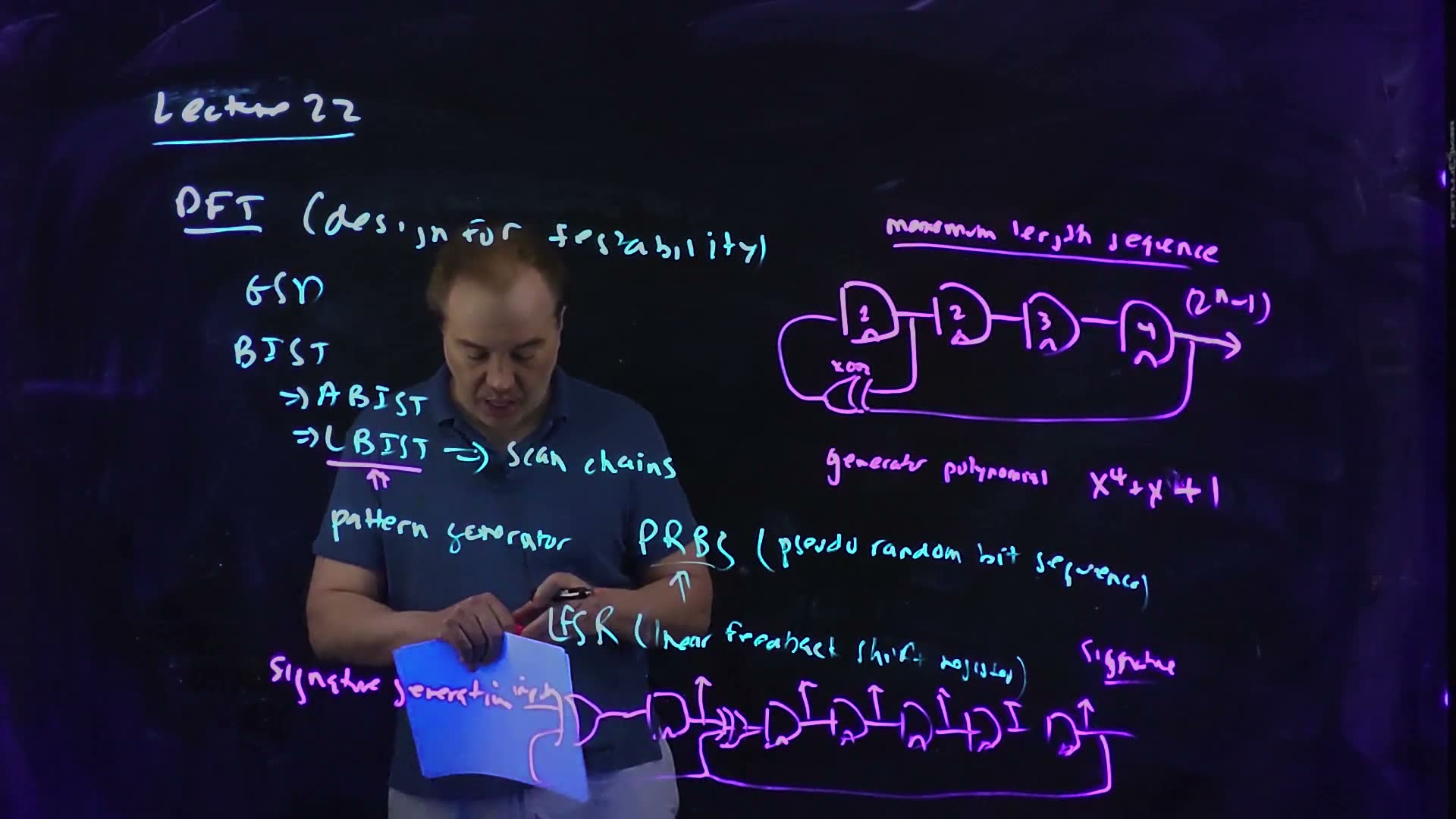
3. Read the signature. At the end the six flip-flops hold the signature: “a kind of compression” (05:17). The small arrows above the flip-flops on the board are the parallel read-out.
4. One compare. The chip compares the signature with the one a simulation of the good circuit predicts. Equal: pass. Different: the circuit is faulty.
5. Good enough (05:17–05:59). “It’s not going to be able to test everything, but … it provides some degree of coverage and it makes the whole thing manageable”: a PRBS in, a signature out, one compare, and an LBIST engine to sequence it.

The board’s signature register board, redrawn (Lecture22 @ 05:08; also at 05:53). The response stream enters at the left: $D_1 = \text{in} \oplus Q_6$ and $D_2 = Q_1 \oplus Q_6$Q6​, the rest shift. The upward arrows read the six bits out in parallel at the end: the signature.

A worked signature

A worked example: a 12-bit response (added; the stream is illustrative)

1. The stream. Take a response of 12 bits, 101100111000, entering first bit first, and reset the register to 000000.

2. The first clocks. Clock 1, input 1: $D_1 = 1 \oplus 0 = 1$1, the rest are 0: 100000. Clock 2, input 0: $D_1 = 0 \oplus 0 = 0$0, $D_2 = Q_1 \oplus Q_6 = 1 \oplus 0 = 1$1: 010000. The feedback first matters when a 1 reaches $Q_6$ (clock 6).

3. The whole run (state $Q_1 \ldots Q_6$ after each clock):

   Clock	1	2	3	4	5	6	7	8	9	10	11	12
   in	1	0	1	1	0	0	1	1	1	0	0	0
   state	100000	010000	101000	110100	011010	001101	010110	101011	000101	110010	011001	111100

   The signature is 111100.

4. A faulty circuit. Suppose a fault flips the fifth response bit (101110111000). The same run ends at 100100: a different signature, so the fault is caught.

5. Why every single error is caught. The register is linear: built from XORs and wires only. So the signature of a stream is the XOR of the signatures of any two streams that XOR to it. The faulty stream is the good one XOR an error stream 000010000000, whose own signature is 011000; and indeed $111100 \oplus 011000 = 100100$100100. An error stream with a single 1 never has signature 000000: the 1 makes the state nonzero, and with no input the register’s step is reversible (each state has exactly one state before it, and 000000’s is 000000), so a nonzero state never becomes 000000. Every single-bit error therefore changes the signature.

6. What it can miss. A long, random error stream lands on the good signature only if its own signature happens to be 000000. Out of $2^6 = 64$ possible signatures, that is about one chance in 64: 1.6 % for six bits. This is aliasing. Real signature registers use 16 to 32 bits, which makes it negligible.

Aliasing probability of an n-bit signatureadded

$$P_{alias} \approx 2^{-n}$$

Holds when: a long error stream whose bits look random, compared with n; a linear (XOR-only) register; single-bit and other short error patterns are always caught by a well-chosen feedback

Memorize: each extra bit halves the chance a fault slips through.

Traps.

• “A matching signature proves the circuit right.” It makes a fault very unlikely, not impossible (aliasing), and it says nothing about faults the patterns never excite.
• No reset. The register must start in a known state, or the good circuit’s signature cannot be predicted.

Check yourself Why does any single wrong bit always change a linear signature?

The faulty stream is the good stream XOR an error stream with one 1 in it, and by linearity its signature is the good signature XOR the error stream’s signature. A single 1 clocked into a reset register makes its state nonzero, and with zeros coming in the register’s step is reversible (only 000000 leads to 000000), so the state never returns to zero. That second signature is never 000000, and the XOR changes the result.

Check yourself Reset the board's register to 000000 and clock in 1, 0, 0. Give the state after each clock.

Clock 1: $D_1 = 1 \oplus Q_6 = 1$1: 100000. Clock 2: $D_1 = 0$0, $D_2 = Q_1 \oplus Q_6 = 1$1: 010000. Clock 3: $D_1 = 0$0, $D_2 = 0$0, $D_3 = Q_2 = 1$1: 001000. With $Q_6 = 0$ throughout, the register is a plain shift register so far.

Check yourself Roughly how many signature bits keep the aliasing probability below one in a million?

$2^{-20} = 9.5 \times 10^{-7}$10−7, just under $10^{-6}$10−6, while $2^{-19}$ is just over: 20 bits.

3. Electromigration: why DC current wears a wire out

You need

The inverter’s currents (Chapter 6). When the output rises, charge flows from $V_{DD}$ through the PFET onto the load; when it falls, the charge flows from the load through the NFET to ground. So the supply wire only ever carries current out of $V_{DD}$VDD​, and the ground wire only ever carries it into ground, while the output wire carries it one way to charge and the other way to discharge.

Current density added. The current per unit of a wire’s cross-section, $J = I/(wt)$ for a wire of width $w$ and thickness $t$t. The same current through a narrower or thinner place has a higher density.

Infant mortality and burn-in (Chapter 22). Some dies carry latent defects that fail early in use. Burn-in runs every die hot (about 85 °C) at a raised supply for a few hours in the factory, so those dies fail there instead of in the field.

The question. A wire carrying current is not inert: over years, a large current can move the metal itself. What is that effect, which wires does it threaten, how does it make a chip fail, and why is burn-in the way to find a wire that will fail early?

From current to a failed wire (board, 07:07–13:12)

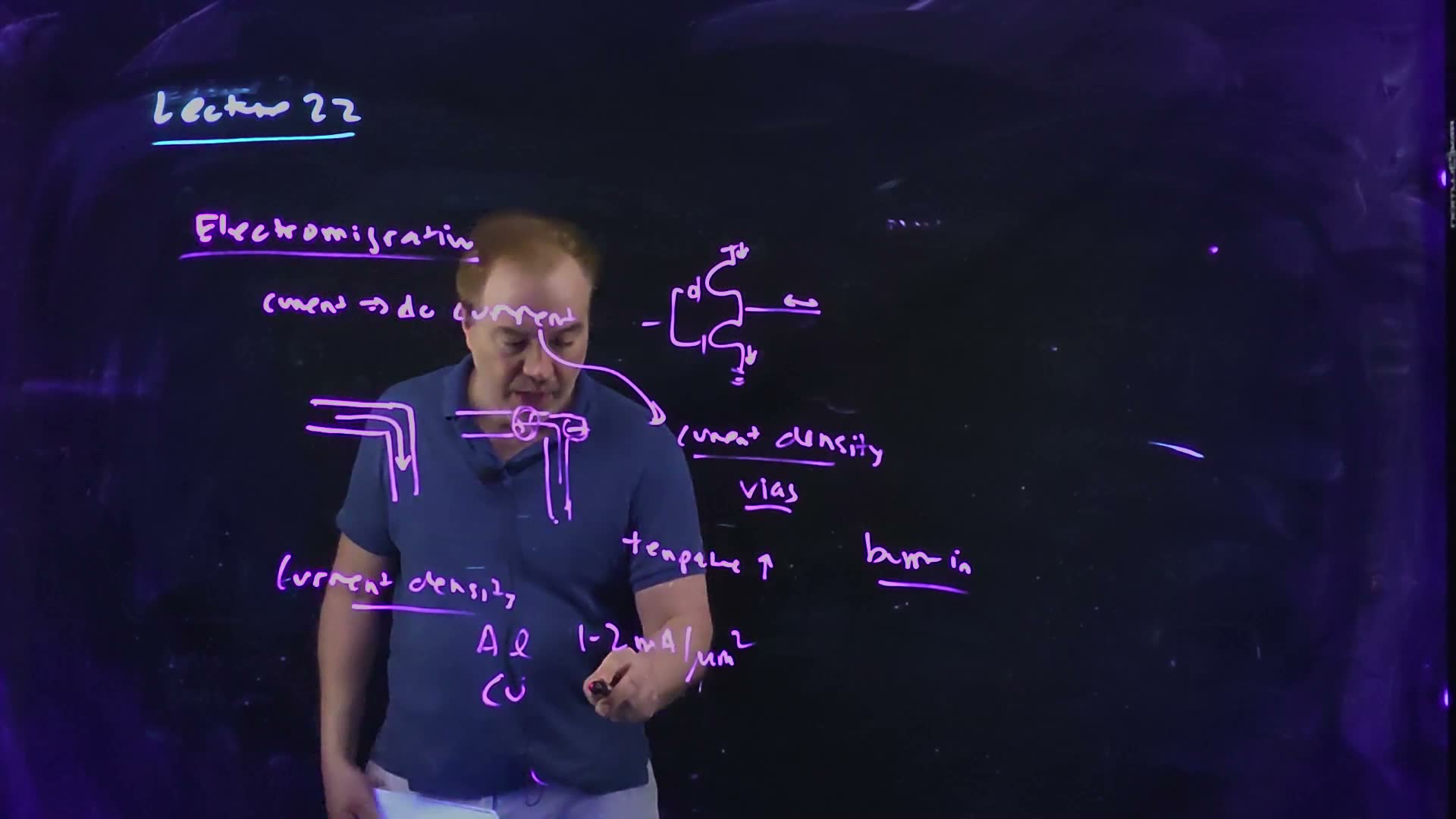
1. The effect board (07:07–07:35). A large current, usually a DC current, pushes the metal ions of the wire along with it. This slow transport of the metal is electromigration: a wear-out mechanism.
2. DC against AC board (08:06–08:31). In an inverter, the supply connections carry current one way all the time: out of $V_{DD}$VDD​, into ground. That is DC. The output wire carries current one way while it charges the load and back while it discharges it: AC, and the ions are pushed back and forth with almost no net motion. “So power connections are often the biggest source” of electromigration.
3. Where it fails board (08:48–09:24; drawn by 12:23). Where current rounds a corner, metal is pulled away from one spot and piled up at another. The depleted spot thins until it becomes a void, an open circuit. The pile becomes a protrusion that can grow into the neighbouring wire and make a short.
4. It is a matter of density board (09:27). Electromigration depends on the current density, the current per cross-section area, not on the current alone. Vias squeeze a wire’s current through a small square, so they are frequent culprits.
5. It is thermally activated board (09:54–10:22). The rate grows exponentially with temperature. That is why burn-in runs hot: it speeds up electromigration so that a weak wire fails in the factory.
6. The defect burn-in catches board (12:39–13:12). A dust particle during fabrication pinches a wire (“this metal”) to a neck. The neck carries the full current through a fraction of the width, so its current density is far higher than designed. Under burn-in it electromigrates open, and the die is rejected before it ships. This is the infant-mortality mechanism that Chapter 22’s burn-in section answers with (FN17-1e).
7. An aside (11:49–12:15). The lecturer calls electromigration “a very bizarre effect”: when someone first described it to him, “I thought they were nuts”, until he saw a time-lapse film of a wire’s metal moving.

Which wires carry DC board, redrawn (Lecture22 @ 12:23; drawn 08:06–08:31). The supply connections carry current one way only, out of $V_{DD}$ and into ground (dc); the output wire carries it to the load and back (ac), so its net push on the metal is about zero.

Where electromigration strikes board, redrawn (Lecture22 @ 10:58, 12:23, 13:12). (a) Current rounding a corner. (b) Metal moved from one spot (a void: an open) to another (a protrusion that can short to the neighbour). (c) A via crowds the current into a small area. (d) A particle pinches a wire to a neck, where the current density is far above the design’s: the defect burn-in finds.

The board (Lecture22 @ 13:12)

Lecture22 @ 13:12The electromigration board: DC current, current density and vias, the corner failures, temperature and burn-in, the dust defect, and the current-density limits.

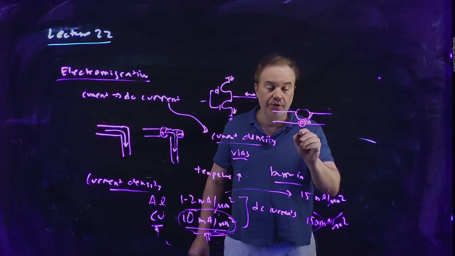
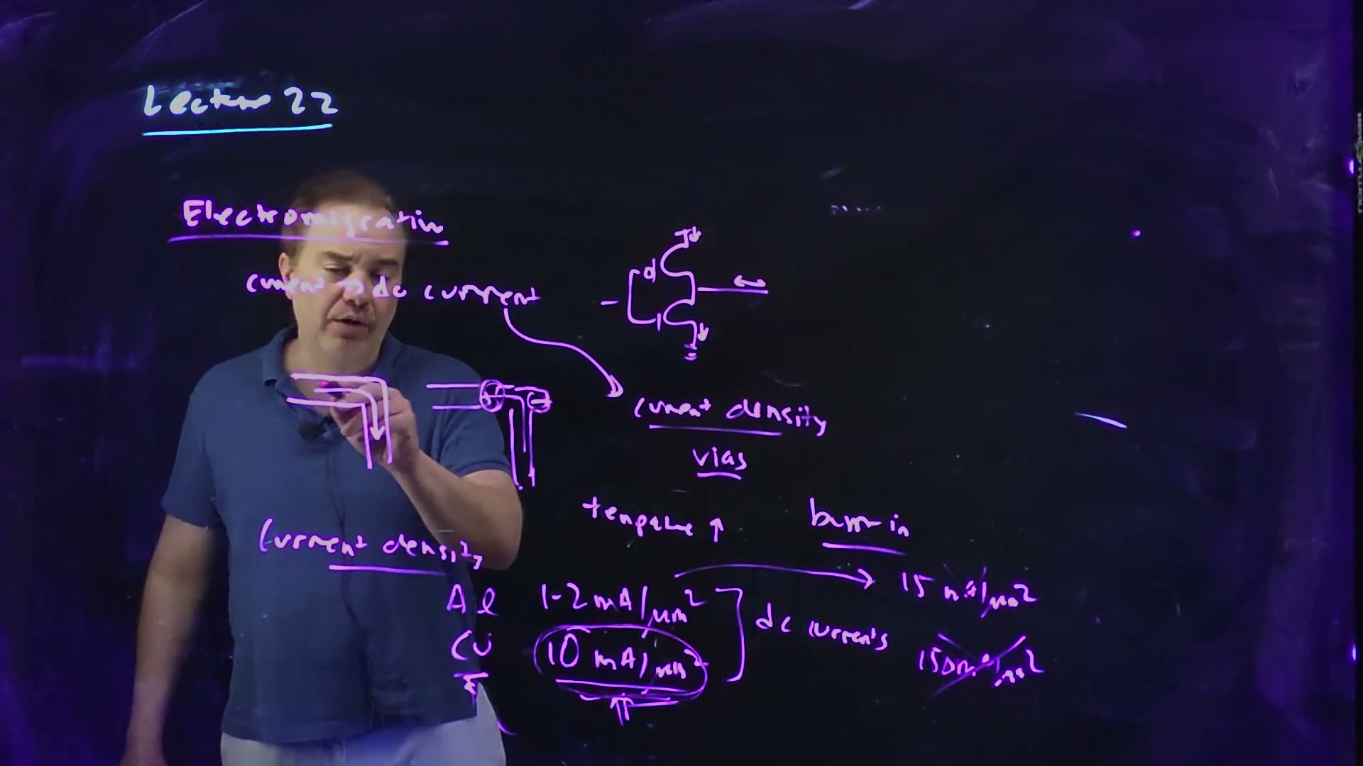
Fair copy of the board above (Lecture22 @ 13:12), mark for mark in its own layout, all in black: one violet pen wrote the topic (“Lecture 22” is the opening board’s cyan title). Nothing is hidden: the lecturer stands behind the strokes (checked against 12:23), and the two wires with the dust particle, top right, are new at 13:12. A long diagonal and a short stroke cross “150 mA/µm²”. They look like a cross-out, but the speech keeps 150 mA/µm² as copper’s AC limit, “so high as to be not even much of an issue” (11:34–11:43), so they are copied as drawn. The hand writes each unit’s slash as a near-vertical bar with µm² below it, as set here. The stroke under “Cu” and the small mark below it run off the lit area and are copied as strokes.

Which wires are at risk

A walk over the inverter drawing above added, wire by wire.

• The $V_{DD}$ strap feeding the inverter’s PFET carries every charging current, always in the same direction: DC. At risk, and more so the more gates it feeds.
• The ground strap carries every discharging current, always into ground: DC. At risk in the same way.
• The output wire carries the same charge out and back each cycle: AC. Its current can be large, but the ions’ net drift cancels, and AC limits are about ten times higher (Section 4). Safe at the densities chips use.
• A via stack on a strap, where the supply drops from a wide upper layer to a lower one, carries DC through a few small squares: the highest density on the path. The worst spot, and the one checked first.

So electromigration is a supply-network problem first: wide straps, many vias in parallel, and no narrow necks on the way from the pads to the cells.

Traps.

• “An output wire’s current averages to zero, so it carries no current.” Its current is large; only the net push on the metal, one way then the other, cancels.
• Electromigration is not IR drop. IR drop is a loss of voltage along a resistive supply (Chapter 21) that slows gates now; electromigration is the wire’s metal moving, which opens or shorts it after months or years.
• The total current is not what matters. A modest current through a narrow neck or a single via can exceed the limit that a wide wire carrying the same current never approaches.

Check yourself Why is a clock net, which switches every cycle, safer from electromigration than the supply strap that feeds its drivers?

The clock wire charges its load and then discharges it: AC, so the metal is pushed one way and then back, with almost no net motion. The strap delivers the charging current of every one of those cycles in the same direction: DC, so its push accumulates.

Check yourself A strap's current density doubles at a constriction, and burn-in runs the chip 60 °C hotter than normal use. Which effect makes the constriction fail during burn-in, and why does it fail before the rest of the strap?

Both act together. Electromigration is thermally activated, growing exponentially with temperature, so burn-in’s heat speeds it up everywhere and moves a weak wire’s failure from years into the factory’s hours. The constriction fails first because there the current density, the quantity electromigration depends on, is twice the strap’s: it was already the weak spot, and the heat only brings its failure forward.

Check yourself Why does the board list vias with current density?

A via joins two wires through a small square, so the whole current of a wide strap passes through a cross-section much smaller than the strap’s. The current density there is high, and electromigration follows current density.

4. Current-density limits and sizing a wire

You need

Electromigration (Section 3). Metal ions are pushed along by current; DC currents (supply straps, ground straps, vias) accumulate the push, AC currents (signal wires) mostly cancel it. The rate depends on the current density $J = I/(wt)$I/(wt), where $w$ is the wire’s width and $t$ its thickness, and it grows exponentially with temperature.

Which wires carry DC (Section 3). Original figure ↑

Copper and aluminium (Chapter 20). Older processes wired chips in aluminium; modern ones in copper, which also has the lower resistivity.

The question. Electromigration sets a limit on current density. What are the numbers, and how does a designer turn them into a wire’s width or a number of vias?

The limits (board, 10:22–11:49)

1. DC limits board (10:40–10:52). Aluminium: 1–2 mA/µm². Copper: about 10 mA/µm², “about a factor of 10” better: another benefit of copper besides its lower resistance.
2. AC limits board (11:23). Far higher: about 15 mA/µm² for aluminium and 150 mA/µm² for copper, “so high as to be not even much of an issue”. The board writes the two numbers; that they are the AC limits is said, not written.
3. The rule for sizing added. Keep $J = I/(wt)$ at or below $J_{max}$Jmax​. With the layer’s thickness $t$ fixed by the process, that sets a minimum area $I/J_{max}$ and a minimum width $I/(J_{max}t)$ (the formula below).
4. The state of things (11:49). Copper “has really helped to solve this”, but supply straps and their vias are still checked against the DC limit.

Sizing for electromigration added. (a) The current density is the current over the cross-section, $J = I/(wt)$I/(wt). (b) Where a strap changes layer, its current divides among an array of vias, each of which may carry only $J_{max}$ times its own small area.

Sizing a wire for electromigrationadded

$$J = \frac{I}{wt} \le J_{max} \quad\Longrightarrow\quad w_{min} = \frac{I}{J_{max}\,t}$$$$N_{via} \ge \frac{I}{J_{max}\,ab}$$

Holds when: a DC current I through a wire of thickness t; J_max the layer's DC limit (Al 1–2, Cu about 10 mA/µm²); for a via array, each via of area a × b carries at most J_max·ab; the AC limits (about 15 and 150 mA/µm²) apply only to signal wires

Derive it: current density is current over area, and the area is width times thickness. Memorize the limits: Al 1–2, Cu ≈ 10 mA/µm² DC; ≈ 15 and 150 AC.

A worked example: a supply strap and its vias (added; values for example)

1. The strap. For example, a supply strap carries 20 mA of DC in a metal layer 0.5 µm thick.
2. In copper ($J_{max}$Jmax​ = 10 mA/µm²). The area must be at least $20/10 =$ 2.0 µm², so the width at least $2.0/0.5 =$ 4.0 µm.
3. In aluminium ($J_{max}$Jmax​ = 1–2 mA/µm²). The area must be 10–20 µm², the width 20–40 µm: five to ten times wider. That is the factor of 10 the board gives copper.
4. The vias. Where the strap drops to the layer below, take copper vias of 0.2 µm × 0.2 µm. Each may carry $10 \times 0.04 =$ 0.40 mA, so the strap needs at least $20/0.40 =$ 50 vias in parallel. One via in the wrong place, carrying the whole strap’s current, would be at fifty times its limit.
5. A signal wire. A copper signal wire 0.1 µm × 0.2 µm may carry only 0.20 mA of DC, but 3.0 mA of AC. Its real current is AC, so it is the higher number that applies, and it is rarely reached.

Check. The two copper numbers agree: a 4.0 µm × 0.5 µm strap has the same 2.0 µm² as fifty 0.04 µm² vias, so both run at exactly the limit.

Traps.

• mA per µm², not per µm. The limit is per unit of cross-section area; a width-only rule ignores the thickness.
• “Million amps.” The lecture’s captions say “million amps per square micron”; the board and the speech say milliamps.
• The AC limit on a supply strap. A strap’s current is DC; its limit is the DC one, ten times lower.
• One via for a strap. A via’s tiny area carries a tiny current; the strap’s current needs an array.

Check yourself Name the two benefits copper brought to supply straps over aluminium.

Its DC electromigration limit is about ten times aluminium’s (10 against 1–2 mA/µm²), so the same current needs a smaller cross-section. And its lower resistivity gives less IR drop for the same width. The lecture (11:03–11:11) calls the first “another big benefit” of copper, beside “lower resistance”: two separate gains, and a strap must satisfy both its electromigration limit and its drop budget.

Check yourself An aluminium strap 0.6 µm thick carries 6 mA of DC at the 2 mA/µm² limit. Find its minimum area and width, and the width in copper at 10 mA/µm².

Area $= 6/2 =$ 3.0 µm²; width $= 3.0/0.6 =$ 5.0 µm. In copper, area $= 6/10 = 0.6$ µm², width $= 0.6/0.6 =$ 1.0 µm: five times narrower.

Check yourself A signal wire's current is AC. Which limit applies, and why is it rarely the binding one?

The AC limit, about 150 mA/µm² in copper: fifteen times the DC limit, because the ions’ push alternates and mostly cancels. A signal wire’s current is set by the load it charges, and long before it nears that density the wire’s RC delay or its driver’s size has become the problem.

5. Synchronous and asynchronous design

You need

The clocked pipeline (Chapter 14). Logic sits between flip-flops on one clock; each stage must finish within one cycle, $T_{cycle} \ge t_{clk\to Q} + t_{logic,max} + t_{setup}$tsetup​. Every stage gets the same cycle, so the clock is set by the slowest stage.

Cycle stealing (Chapter 14). With transparent latches instead of flip-flops, a slow stage can borrow time from the next, so the cycle is set closer to the average than to the worst stage.

The question. Every circuit so far has run on a clock. Is there another way to sequence logic, what does it gain, and why does almost every chip still use a clock?

Two ways to sequence logic (board, 14:07–17:21)

1. Synchronous board (14:07–14:40). The logic is “sequenced by a special control signal”, the clock, and that signal is global: one clock reaches every flip-flop.
2. Asynchronous board (15:00–15:47). There is no clock. The control signals are local: each stage talks only to its neighbours by handshaking, most commonly a “four-phase handshaking protocol” (15:13). added In a four-phase handshake the sender raises request when its data is ready; the receiver takes the data and raises acknowledge; the sender drops request; the receiver drops acknowledge, and the pair is ready for the next item.
3. What it costs (15:39). “The control overhead is high”: added two extra wires and four transitions for every transfer, and the circuitry to make them.
4. What it gains (15:55–16:24). No global clock to distribute, so none of the problems of Sections 6–10. And each stage proceeds as soon as it is done, so the pipeline runs at the average stage delay rather than the worst case.
5. Why the clock wins (16:24–17:19). Synchronous designs recover part of that gain with cycle stealing, and asynchronous techniques (self-timed circuits) are used inside synchronous chips where they pay. Synchronous design “tends to win the day” because it is so much easier to design and verify.

Synchronous against asynchronous sequencing added, after the board (Lecture22 @ 17:21). (a) One global clock sequences every register. (b) A four-phase handshake: (1) req rises with the data, (2) ack rises once the receiver has it, (3) req falls, (4) ack falls; only then can the next item go.

The board (Lecture22 @ 17:21)

Lecture22 @ 17:21Synchronous design, sequenced by one global clock; asynchronous design, with local control signals and handshaking.

Fair copy of the board above (Lecture22 @ 17:21), mark for mark in its own layout, all in black: a pale blue pen wrote the board (“Clocking” is the heading in the pink-violet pen, “Lecture 22” the opening board’s cyan title). The start of “control signals” and the arrow before it, behind the lecturer’s hand, are restored from 17:44. “sequences”† is a slip for “sequenced”: the speech says “sequenced by a special control signal” (14:25).

A worked example: three stages (added; illustrative delays)

1. The stages. Three logic stages take 300, 500 and 400 ps. Follow one data item through all three.
2. Synchronous. With flip-flops, every stage gets the cycle the slowest needs: 500 ps of logic plus the flip-flop overhead ($t_{clk\to Q} + t_{setup}$tclk→Q​+tsetup​). With 100 ps of overhead, for example, the clock is 600 ps per stage, and the item takes $3 \times 600 =$ 1,800 ps to pass the three stages.
3. Asynchronous. Each stage hands its result on when it is done. With 150 ps of handshake per stage, for example, the item takes $300 + 500 + 400 + 3 \times 150 =$ 1,650 ps: on average $(300 + 500 + 400)/3 =$ 400 ps of logic plus 150 ps, 550 ps per stage.
4. The comparison. The asynchronous pipeline is faster, but only by 50 ps a stage, and the margin vanishes if the handshake costs a little more or if the stages are better balanced.
5. What the average does not set added. With these fixed delays, a simple asynchronous pipeline can accept a new item only as fast as its slowest stage finishes a transfer, $500 + 150 =$ 650 ps, against the clock’s 600 ps: its rate is no better. The average-delay gain the lecture names is real when a stage’s delay changes from one data item to the next: each item then takes only as long as it needs, while a clock must always allow for the worst case.

Traps.

• Two meanings of “asynchronous”. Here it is a design style with no clock. Chapter 13’s “asynchronous set and reset” are inputs that act on a flip-flop without waiting for the clock edge.
• “Asynchronous is always faster.” It runs at the average delay plus the handshake; with balanced stages, the clock’s single overhead can win.

Check yourself What does the four-phase handshake's return to zero cost?

Two of its four transitions (req falling, then ack falling) carry no data: they only reset the wires for the next transfer. Each transfer therefore waits for two extra wire delays and two extra logic responses, which is the control overhead the lecture names.

Check yourself In the example, suppose the stages are retimed to 400, 400 and 400 ps. Compare the two pipelines with the same overheads.

Synchronous: $400 + 100 =$ 500 ps per stage. Asynchronous: average $400 + 150 =$ 550 ps. With balanced stages, the average equals the worst, the asynchronous design loses its only advantage, and the handshake makes it slower.

6. Judging a clock network: skew, jitter, power and latency

You need

What skew costs (Chapter 14). Between a launching and a capturing flip-flop, let the capturing clock arrive later by a signed skew $\delta$δ. The long path then needs $t_{clk\to Q} + t_{logic,max} + t_{setup} \le T_{cycle} + \delta$δ, and the short path needs $t_{clk\to Q} + t_{logic,min} \ge t_{hold} + \delta$δ. A skew that helps one check hurts the other. Jitter, a clock edge that moves from one cycle to the next, is taken as skew in whichever direction hurts.

The short path with a late capture clock (Chapter 14, after Lecture13): the skew adds to the hold requirement. Original figure ↗

The supply sensitivity of delay (Chapter 21; FS1’s FN10-6). Write a gate’s delay as $t$ and define $S_V = (V_{DD}/t)(\partial t/\partial V_{DD})$(VDD​/t)(∂t/∂VDD​), the fractional change of delay per fractional change of supply. (Chapter 21 and FS1 call it $S$S; this chapter writes $S_V$ to keep it apart from the subthreshold slope $S$ of Sections 12–16.) For a small change, $\Delta t/t \approx S_V\,\Delta V_{DD}/V_{DD}$SV​ΔVDD​/VDD​. With the velocity-saturated delay $t \propto V_{DD}/(V_{DD} - V_T)$ (Chapter 5), $S_V = -V_T/(V_{DD} - V_T)$VT​): negative, since a lower supply is slower. Only the gates’ (silicon) delay depends on $V_{DD}$VDD​; a wire’s RC delay does not.

The question. Chapter 14 took the skew as given. Where does it come from? What should a clock network be judged by, and why does the lecture single out its latency, which affects every flip-flop the same way?

The four metrics (board, 17:55–21:35)

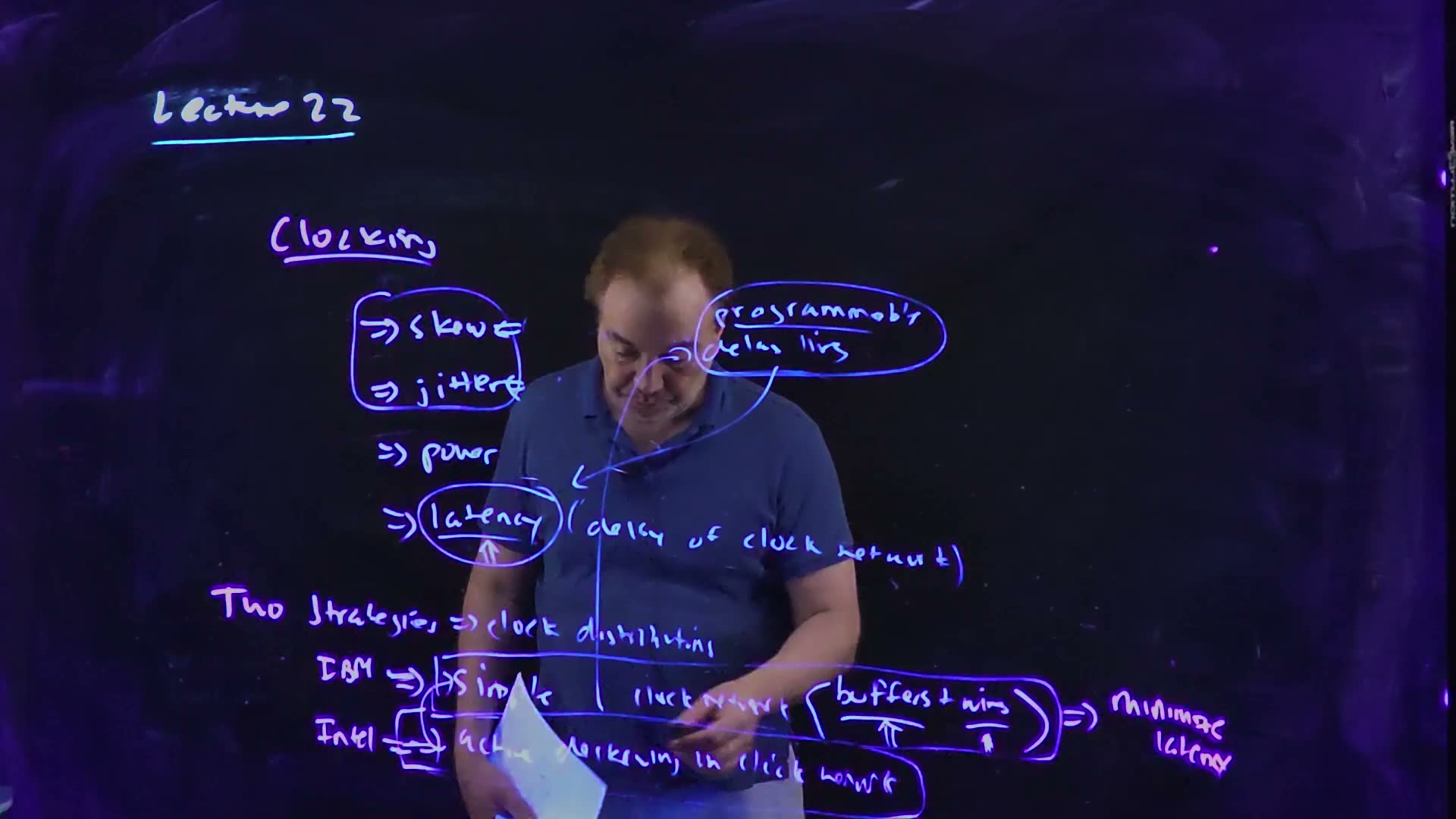
1. The ideal (18:03–18:29). Drive the clock from one point and reach every flip-flop at exactly the same instant: zero skew.
2. Skew board: “static differences in arrival time”. Two flip-flops’ clocks arrive at different times, by the same amount every cycle.
3. Jitter board: “transient differences in arrival time”. The clock edge “can move around”: “one cycle can be shorter, another cycle can be longer”.
4. Power board. The clock net switches every cycle and drives every flip-flop, so it is one of the biggest consumers on the chip (Sections 8 and 12).
5. Latency board: “the delay of the clock network”, from its root to a leaf flip-flop. Call it $t_L$ added.
6. Why latency matters (19:43–20:16). If every flip-flop’s clock arrives $t_L$ late, the edges still arrive together; so why care? Because “if I have a large latency in my clock distribution network, that’s going to translate into skew and jitter.”
7. Where the spread comes from (20:16–21:13). Across the die, process, supply and temperature are not uniform. A static difference (a slow region, a lower local supply, a hot spot) makes two nominally equal paths differ by the same amount every cycle: skew. A transient one (supply noise that changes from cycle to cycle) makes the same path differ from one edge to the next: jitter.
8. So keep it short (21:13–21:35). “The more latency I have, the more sensitivity I have in my clock network to transient and static variation … process, temperature, and voltage to produce skew and jitter.”

Latency turns variation into skew and jitter added, after the board’s definitions (Lecture22 @ 21:57). (a) Every leaf’s clock comes $t_L$ after the root’s. One buffer on B’s branch sees a lower supply. (b) A static difference delays clk_B by the same $\delta$ every cycle: skew. A supply that varies from cycle to cycle moves clk_B’s edge within a band: jitter.

The board (Lecture22 @ 21:57)

Lecture22 @ 21:57The four metrics of a clock network: skew, jitter, power and latency, with the board's definitions. This is the only frame that shows the skew and jitter definitions; they are wiped by 24:48.

Fair copy of the board above (Lecture22 @ 21:57), mark for mark in its own layout, all in black: a pale blue pen wrote the list (“Clocking” is the pink-violet heading, “Lecture 22” the opening board’s cyan title). “skew”, washed out behind the lecturer’s head, is restored from 20:41. The four ditto marks after “transient” repeat “differences in arrival time”. “Two strategies ⇒ clock d” is still being written; it becomes “clock distribution” by 22:29 and is copied only as far as written here. This is the only frame with the skew and jitter definitions: they are wiped by 24:48.

How much skew and jitter a latency makes

The lecture argues in words. One added step added puts a size on it, using only Chapter 21’s sensitivity.

From a supply change to a spread in arrival time (added)

1. One buffer. A fractional supply change $\Delta V_{DD}/V_{DD}$ changes a buffer’s delay by the fraction $S_V\,\Delta V_{DD}/V_{DD}$ (Chapter 21).
2. A whole path. Every buffer on the path from the root to a leaf sees the same change, so the path’s delay $t_L$ changes by the same fraction: $\Delta t_L \approx S_V\,(\Delta V_{DD}/V_{DD})\,t_L$SV​(ΔVDD​/VDD​)tL​. The change is a fixed share of the latency.
3. Static: skew. If the change is static and only one branch sees it, that branch’s leaves arrive later by $\lvert\Delta t_L\rvert$ every cycle.
4. Transient: jitter. If the change is a droop that comes and goes, the same leaf’s edge moves by $\lvert\Delta t_L\rvert$ between cycles.
5. The result. Both are proportional to the latency. Halve $t_L$ and the same variation makes half the skew and half the jitter.

Skew and jitter from latencyadded

$$t_{skew},\ t_{jitter} \;\approx\; \lvert S_V\rvert\,\frac{\Delta V_{DD}}{V_{DD}}\,t_L, \qquad S_V = -\frac{V_T}{V_{DD} - V_T}$$

Holds when: a small variation (a few percent) in the supply, or in any parameter that changes every buffer's delay by the same fraction; all buffers on the path equally sensitive; for skew a static difference between branches, for jitter a change between edges; t_L is the silicon (buffer) part of the latency, since wire RC does not move with V_DD

Derive it in three lines: one buffer’s $\Delta t/t \approx S_V\,\Delta V/V$SV​ΔV/V; every buffer on the path sees it; sum along the path, so $\Delta t_L \approx S_V(\Delta V/V)t_L$SV​(ΔV/V)tL​. FS1 uses exactly this for FN10-6c (FS1, FN10-6c); that part is solved there and not here.

A worked example: a 1 ns network and a 400 ps one (added; values for example)

1. The devices. For example, $V_{DD}$ = 1.0 V and $V_T$ = 0.3 V. Then $S_V = -0.3/(1.0 - 0.3) =$ −0.4286: a 1 % lower supply makes every buffer 0.43 % slower.
2. A 1 ns network, static. One side of the die sits at a supply 5 % lower. The leaves there arrive later by $0.4286 \times 0.05 \times 1000$ ps $=$ 21.4 ps: skew.
3. A 1 ns network, transient. A droop of 8 % comes and goes with the activity. The edge moves by $0.4286 \times 0.08 \times 1000$ ps $=$ 34.3 ps: jitter. The exact model, $t \propto V/(V - V_T)$ evaluated at 0.92 V against 1.0 V, gives 38.7 ps: first order is a little low for an 8 % change.
4. A 400 ps network. The same variations give $0.4286 \times 0.05 \times 400 =$ 8.6 ps of skew and $0.4286 \times 0.08 \times 400 =$ 13.7 ps of jitter (exactly 15.5 ps): 0.4 times as much, in proportion to the latency.

Skew and jitter grow in proportion to the latency added, computed from $\Delta t = \lvert S_V\rvert(\Delta V/V)t_L$ with $S_V = -0.4286$ ($V_{DD}$VDD​ = 1.0 V, $V_T$ = 0.3 V): an 8 % transient droop (solid, jitter) and a 5 % static difference (dashed, skew). The 400 ps network has 0.4 times the 1 ns network’s skew and jitter.

Check. At the 1 ns network, the ratio of jitter to skew is $34.3/21.4 = 1.6$1.6, the ratio of the two variations ($8/5$8/5): the formula is linear in the variation as well as in the latency.

Why it matters added. Every picosecond of skew and jitter comes off the setup margin of the long path and the hold margin of the short path (Chapter 14). A lower latency also needs fewer buffer stages, which cost clock power.

The four metrics of a clock networkboard

• skew: static differences in arrival time;
• jitter: transient differences in arrival time;
• power: the clock net switches every cycle;
• latency: the delay of the clock network, root to leaf.

Holds when: definitions as the lecture writes them

Memorize the four, with the lecture’s argument in one line: latency turns process, voltage and temperature variation into skew and jitter, so keep it low. That is FN17-1d’s answer.

Traps.

• “Only skew matters.” Jitter cannot be tuned out by design, because it changes every cycle.
• One buffer’s delay. The spread scales with the whole root-to-leaf latency, not with the delay of the last buffer.
• “A latency that is the same everywhere is harmless.” Only while nothing varies; every variation acts on all of it.
• $S_V$ and $S$S. The supply sensitivity $S_V$ is a negative number without units; the subthreshold slope $S$ is in mV per decade.

Check yourself Name one static and one transient source of variation, and the metric each produces.

Static: a process gradient across the die, a region with a lower average supply (IR drop), or a hot spot; each makes one branch consistently slower: skew. Transient: supply noise from $L\,dI/dt$ when a block switches on; it slows the same branch on some cycles and not others: jitter.

Check yourself A 1.2 ns clock tree at 1.0 V (V_T = 0.3 V) sees a 6 % droop on one branch only, coming and going. Estimate the jitter between leaves on the two branches; then for a 600 ps tree.

$S_V = -0.3/0.7 = -0.4286$−0.4286. The droop slows the drooping branch by $0.4286 \times 0.06 \times 1200$ ps $=$ 30.9 ps while the other is unchanged, so the edges on the two branches move apart by that much from cycle to cycle. Halving the latency halves it: 15.4 ps.

Check yourself Why does a lower supply, closer to V_T, make the same network jitter more?

$\lvert S_V\rvert = V_T/(V_{DD} - V_T)$ grows as $V_{DD}$ approaches $V_T$VT​: at 1.0 V it is 0.43, at 0.6 V it is 1.0. Each buffer’s delay becomes more sensitive to the same fractional droop, so the same latency turns it into more jitter.

7. Two strategies: minimum latency or active deskew

You need

Latency into skew and jitter (Section 6). A variation that changes every buffer’s delay by a fraction $\epsilon$ moves a leaf’s clock by $\epsilon\,t_L$ϵtL​, where $t_L$ is the root-to-leaf latency; for the supply, $\epsilon \approx \lvert S_V\rvert\,\Delta V_{DD}/V_{DD}$ with $S_V = -V_T/(V_{DD} - V_T)$VT​). Static variation gives skew; transient variation gives jitter.

Skew and jitter in proportion to the latency (Section 6). Original figure ↑

A feedback loop added (circuits background). A loop measures an error (here, the difference between two clocks’ arrival times), and a controller adjusts something (here, a delay) to drive the error toward zero. It can follow changes slower than its own response time, not faster ones.

The question. Given that latency breeds skew and jitter, there are two ways to fight them: build the network so its latency is small, or measure the skew and cancel it. What does each involve, and what can each not do?

Two strategies (board, 21:52–26:48)

1. A simple clock network board (21:52–23:47). Only buffers and wires. (The lecturer starts to call it “passive”, then corrects himself: the buffers are active devices, so “let me just call it simple clock network”.) Many levels of buffers are still needed, because the total load of all the flip-flops is enormous.
2. Its goal: minimize latency board (24:11–24:38). “The best way to deal with skew and jitter in my clock distribution network is to just minimize the latency … Just keep the latency low.”
3. Active deskewing board (23:47–25:36). Build programmable delay lines into the network, measure the skew between regions, and set the delays to cancel it. With a feedback loop running all the time, it can also track some slow, transient variation.
4. Its cost (25:41). “The problem with these delay lines, of course, is that they’re adding latency.” The delay lines are themselves buffers whose delay varies, and the loop must correct that too.
5. Who did which board (26:00–26:48). As the lecturer recalled it at the recording: IBM used the simple network, Intel active deskewing. Both still build their networks from buffers and wires (Sections 8–10).
6. What deskew can and cannot fix added. It removes static skew and slow drift (process, temperature, the average supply). It cannot remove jitter faster than its loop responds, and the latency its delay lines add makes that jitter larger.

The two strategies added, after the board (Lecture22 @ 27:16). (a) A simple network of buffers and wires, designed for the least latency $t_L$tL​. (b) Active deskew: programmable delay lines ($\Delta$Δ) before the leaves, a phase detector (PD) comparing two regions’ clocks, and feedback that sets the delays to cancel the difference.

The board (Lecture22 @ 27:16)

Lecture22 @ 27:16Two strategies: IBM's simple network of buffers and wires, which minimizes latency, and Intel's active deskewing with programmable delay lines.

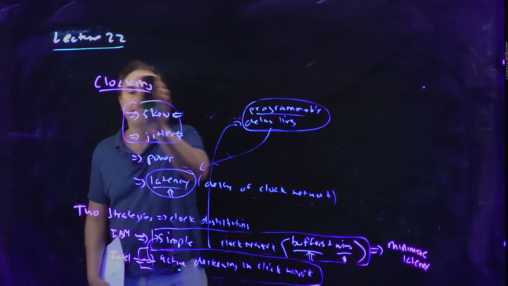
Fair copy of the board above (Lecture22 @ 27:16), mark for mark in its own layout, all in black: one pale blue pen wrote the board. The underline of “Lecture 22” is the cyan title pen, and “minimize latency” is the pink-violet pen, a single note written in the run of the blue writing (24:11–24:38), not a separate layer. The definitions of skew and jitter were wiped earlier; only their arrows remain. The right side of the skew and jitter box and the start of “Clocking”, under the lecturer’s hand, and “Intel”, under his sheet of paper, are restored from 26:48. On the last line “clock network” is set a size smaller so that it stays inside its box.

A worked example: what deskew buys (added; values for example, from Section 6)

1. The network. Section 6’s 1 ns network at 1.0 V ($S_V = -0.4286$SV​=−0.4286): a 5 % static difference gives 21.4 ps of skew, an 8 % droop 34.3 ps of jitter.
2. Deskew it. The loop cancels the static 21.4 ps. Suppose its delay lines add 200 ps to every path, for example. The latency is now 1.2 ns.
3. The jitter grows. The droop comes and goes faster than the loop follows, so it is not cancelled; it now acts on 1.2 ns: $0.4286 \times 0.08 \times 1200$ ps $=$ 41.1 ps, up from 34.3 ps.
4. The simple alternative. A 400 ps network with no loop has 8.6 ps of skew and 13.7 ps of jitter (Section 6). If such a network can be built, it beats the deskewed one on both counts.

Traps.

• “Deskew removes jitter.” It removes what its loop can follow: static skew and slow drift. Fast jitter remains, and grows with the added latency.
• Forgetting the delay line’s own latency. Every programmable delay is a chain of buffers on the clock path.

Check yourself Why do both companies still care about the buffer-and-wire network underneath?

Deskewing only corrects what the network does wrong. The network still carries the clock with all its latency to every flip-flop; its latency still sets the jitter the loop cannot follow, and its power is the same. A deskewed network that starts from a long latency ends with a lot of jitter.

Check yourself A deskew loop's delay lines add 300 ps to a 700 ps network at 1.0 V (V_T = 0.3 V). Find the jitter from an 8 % droop before and after.

$\lvert S_V\rvert = 0.4286$0.4286. Before: $0.4286 \times 0.08 \times 700$ ps $=$ 24.0 ps. After, with 1000 ps of latency: $0.4286 \times 0.08 \times 1000 =$ 34.3 ps. The loop has removed the static skew, at the price of 43 % more jitter.

8. Clock grids

You need

Power grids (Chapter 21). The supply is spread over the chip by a mesh of straps on every metal layer. Many parallel paths between any two points give a low resistance and a low inductance, so the voltage is nearly the same everywhere.

A power grid (Chapter 21): many parallel paths, low R and L. Original figure ↗

Driving a big load (Chapter 8). A small signal drives an enormous capacitance through a chain of inverters, each a few times (about four times) larger than the one before.

Clock power (Chapter 6). Charging a capacitance $C$ to $V_{DD}$ draws $CV_{DD}^2$ from the supply. A clock node rises once every cycle, so a clock network of capacitance $C_{clk}$ at frequency $f$ burns $P = C_{clk}V_{DD}^2 f$Cclk​VDD2​f.

The question. A supply grid keeps the voltage nearly equal everywhere because it is a mesh with low resistance. Could a clock be distributed the same way, so that it arrives nearly at once everywhere? What does such a clock grid buy, and what does it cost?

The clock grid (board, 27:52–31:57)

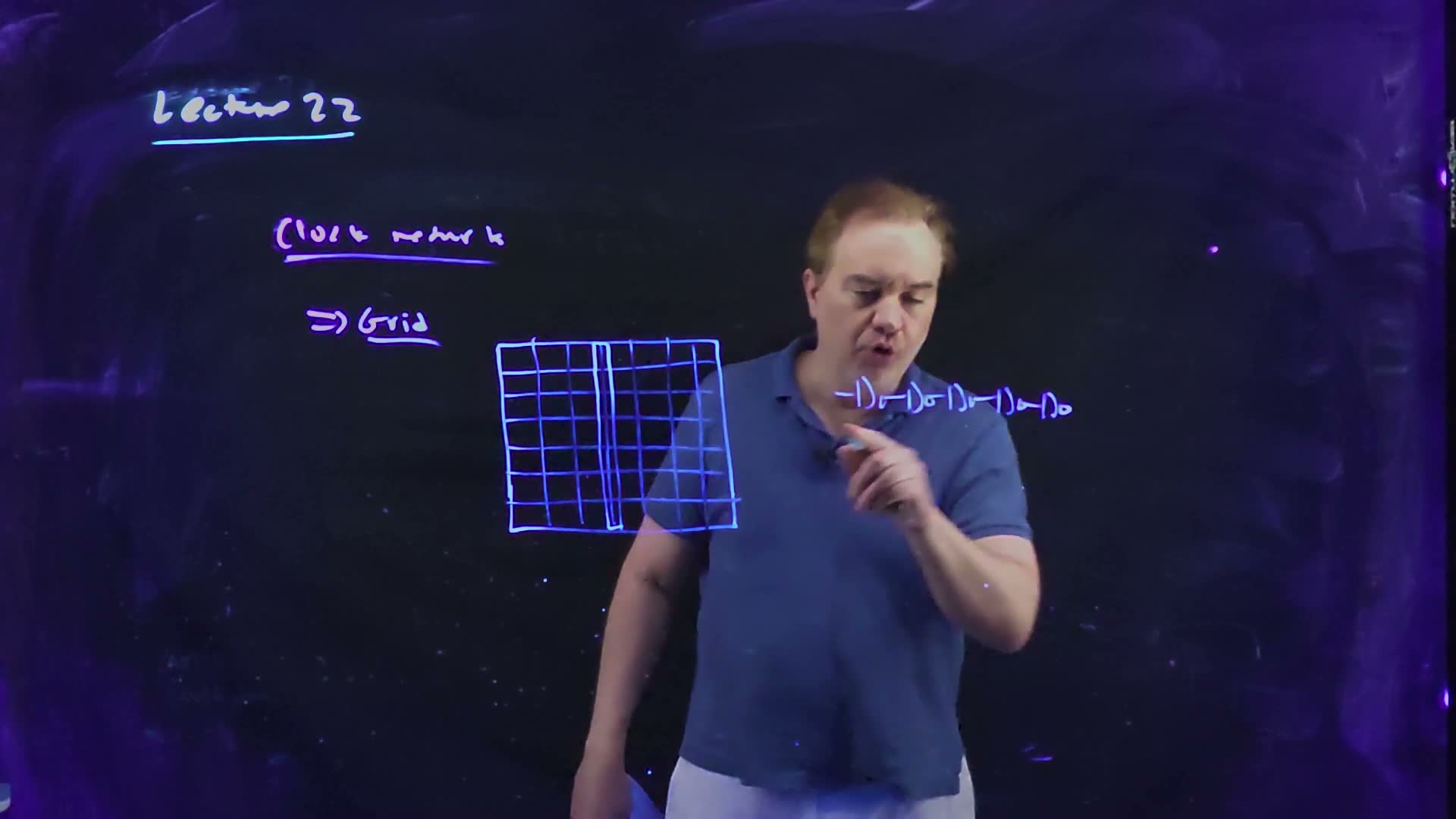
1. Borrow the power grid’s idea (27:52–28:20). Low resistance and inductance spread the clock uniformly across the chip: a grid.
2. The DEC Alpha board (28:28–29:42). The quintessential example, as the lecturer recalled it: the DEC Alpha processor of the early 1990s used one grid for the whole chip. All the buffering sat up front, a chain of inverters growing in size, and the final inverter was “distributed over the entire spine”: one huge driver laid out along a strip across the middle of the chip, with an effective width the lecturer recalls as “like two centimetres or something”.
3. Why it has little skew (29:42–30:09). There is little RC or LC delay across the grid, so when the spine switches, “this whole grid would come along with it”: every flip-flop sees nearly the same edge, out to the periphery.
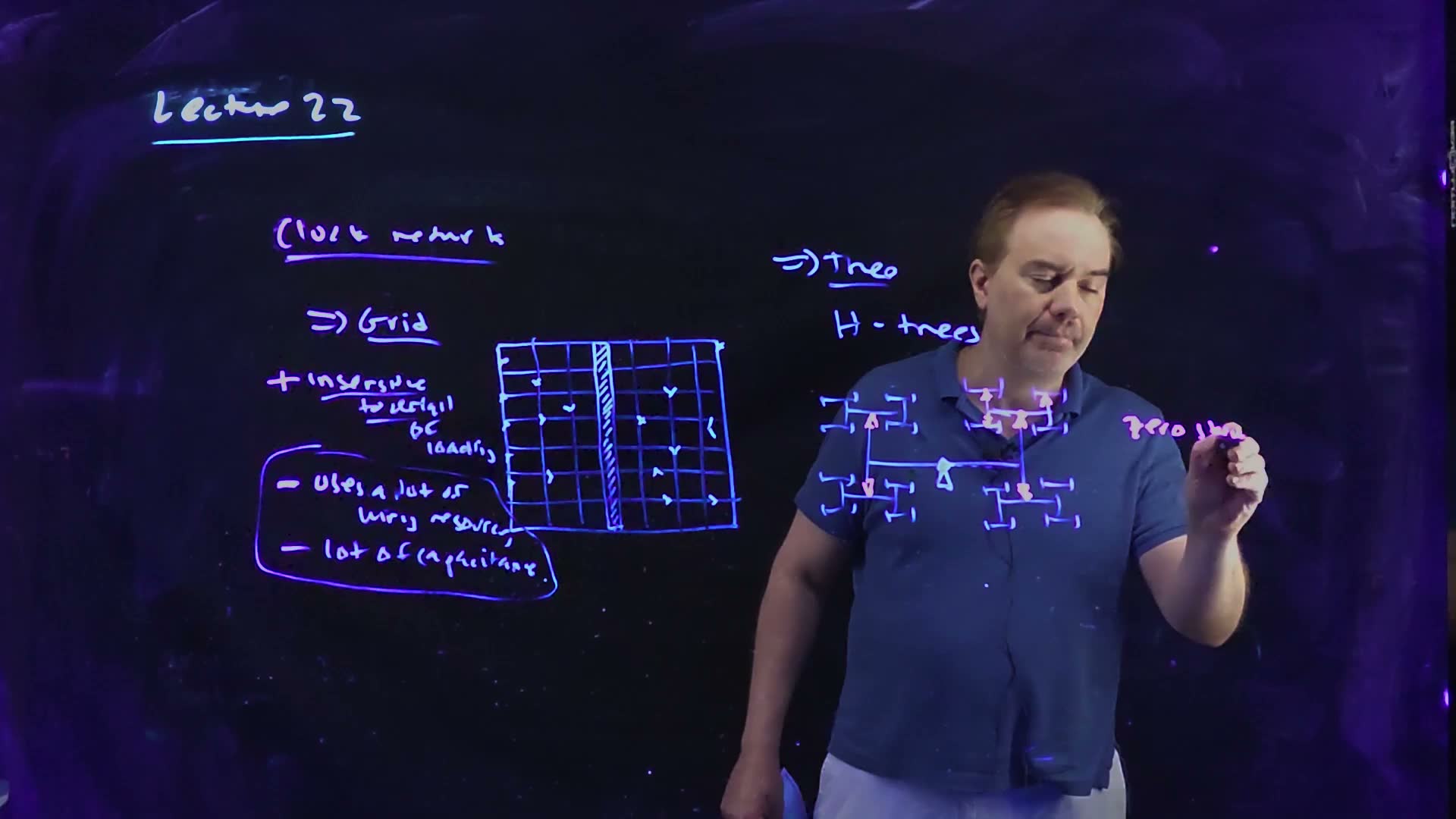
4. Its plus board (30:41–31:35). Insensitive to the details of loading: a flip-flop can be added late, anywhere, without retuning anything.
5. Its two minuses board. It uses a lot of wiring resources, and it has a lot of capacitance, so it is power-hungry.
6. Since then (31:53). As the lecturer told it, pure grids have not been used much since the Alpha.

A clock grid board, redrawn (Lecture22 @ 31:57; begun at 29:04). A chain of growing inverters drives one huge final driver laid along the hatched spine (the DEC Alpha’s, as the lecturer recalls it, “like two centimetres” wide); the spine drives the whole grid; the small marks are flip-flops tapping the grid wherever they sit.

The board (Lecture22 @ 31:57)

Lecture22 @ 31:57The clock grid: insensitive to loading, but heavy in wiring and capacitance; the spine and the buffer chain that drives it.

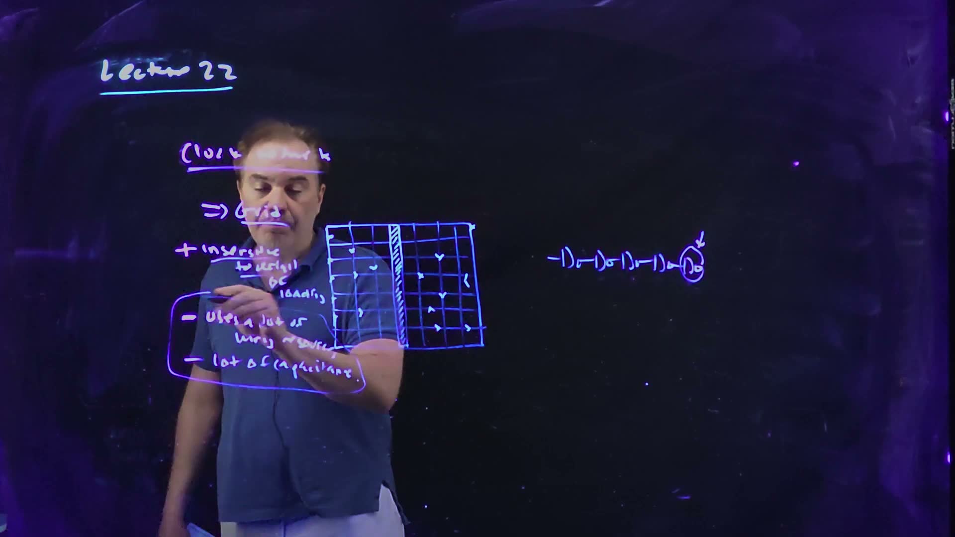
Fair copy of the board above (Lecture22 @ 31:57), mark for mark in its own layout, all in black: one pale blue pen wrote the board, and the underline of “Lecture 22” is the cyan title pen. “network”, “Grid” and the left of the list, behind the lecturer’s head and arm, are restored from 37:14, where the left half is unchanged and clear. The hatched strip is the spine, the distributed final inverter; the small marks at the nodes are flip-flops tapping the grid. “wiring resources” starts a little left of the board’s, for the wider typeset words.

A worked example: the price of a grid (added; values for example)

1. The chip. A square die $D$ = 10 mm on a side, with a clock grid of pitch $p$ = 1.25 mm.
2. The wire. The grid has $D/p + 1 = 9$ lines in each direction, each 10 mm long: $2D(D/p + 1) = 2 \times 10 \times 9 =$ 180 mm of clock wire.
3. Its capacitance. At 0.2 fF/µm (an illustrative wide clock wire), $180{,}000\ \mu\text{m} \times 0.2\ \text{fF}/\mu\text{m} =$ 36 pF, before a single flip-flop is connected.
4. Its power. At 1 V and 2 GHz, $C V^2 f = 36\ \text{pF} \times 1\ \text{V}^2 \times 2\ \text{GHz} =$ 72 mW for the bare grid.

Check. Each line of the grid is a full 10 mm long, and nine lines each way make 18 lines: 180 mm, as counted.

Traps.

• “A grid has no skew.” It has little, because the resistance between its taps is low, not zero; the corners farthest from the spine still lag.
• “Its capacitance is free because it is only wire.” Every millimetre switches every cycle; the wire is a large share of the clock’s power.

Check yourself Why is a grid insensitive to where the loads are?

Between any two points there are many parallel paths with low resistance, so a flip-flop added at one node draws its charge from all around it, and the node’s delay barely moves. In a tree, by contrast, the same load hangs on one branch and slows only that branch.

Check yourself Halve the grid pitch in the example to 0.625 mm. How much clock wire, and how much power for the bare grid?

$D/p + 1 = 17$ lines each way: $2 \times 10 \times 17 =$ 340 mm, so 68 pF and 136 mW at 1 V and 2 GHz: 1.89 times as much: not quite twice, because the number of lines goes from 9 to 17 each way, not to 18.

9. H-trees, and tuning wire for wire

You need

The delay of a driven load (Chapter 20). A driver of resistance $R$ charging a lumped capacitance $C$ has an Elmore delay $RC$RC; add $\Delta C$ to the load and the delay grows by $R\,\Delta C$RΔC.

Latency into skew (Section 6). A variation that changes a delay by a fraction acts on the whole delay it touches: $\Delta t \approx \lvert S_V\rvert(\Delta V_{DD}/V_{DD})\,t$ for the supply, with $S_V = -V_T/(V_{DD} - V_T)$VT​).

Only silicon moves with the supply (Chapter 21). A buffer’s delay depends on $V_{DD}$VDD​; a wire’s RC delay does not, though it does change with the wire’s own process corner and temperature.

Latency turns variation into skew and jitter (Section 6). Original figure ↑

The question. Instead of a grid, a clock can be sent along a tree whose every path from the root to a leaf is the same. How is such a tree built, why is it sensitive where the grid was not, how is it tuned, and what does it save?

The H-tree (board, 32:21–36:56)

1. Nested H’s board (32:21–33:18). Draw an H across the chip with the clock driven at its centre. At each of its four tips, draw a smaller H, and so on. By symmetry, “the wire length … to any leaf node is always exactly the same”: the ideal of zero skew, built into the geometry.
2. Buffers in the tree board (33:18–33:40). The buffers are spread through the tree (the lecturer calls them sector buffers), at the centre of each H, not all at the root.
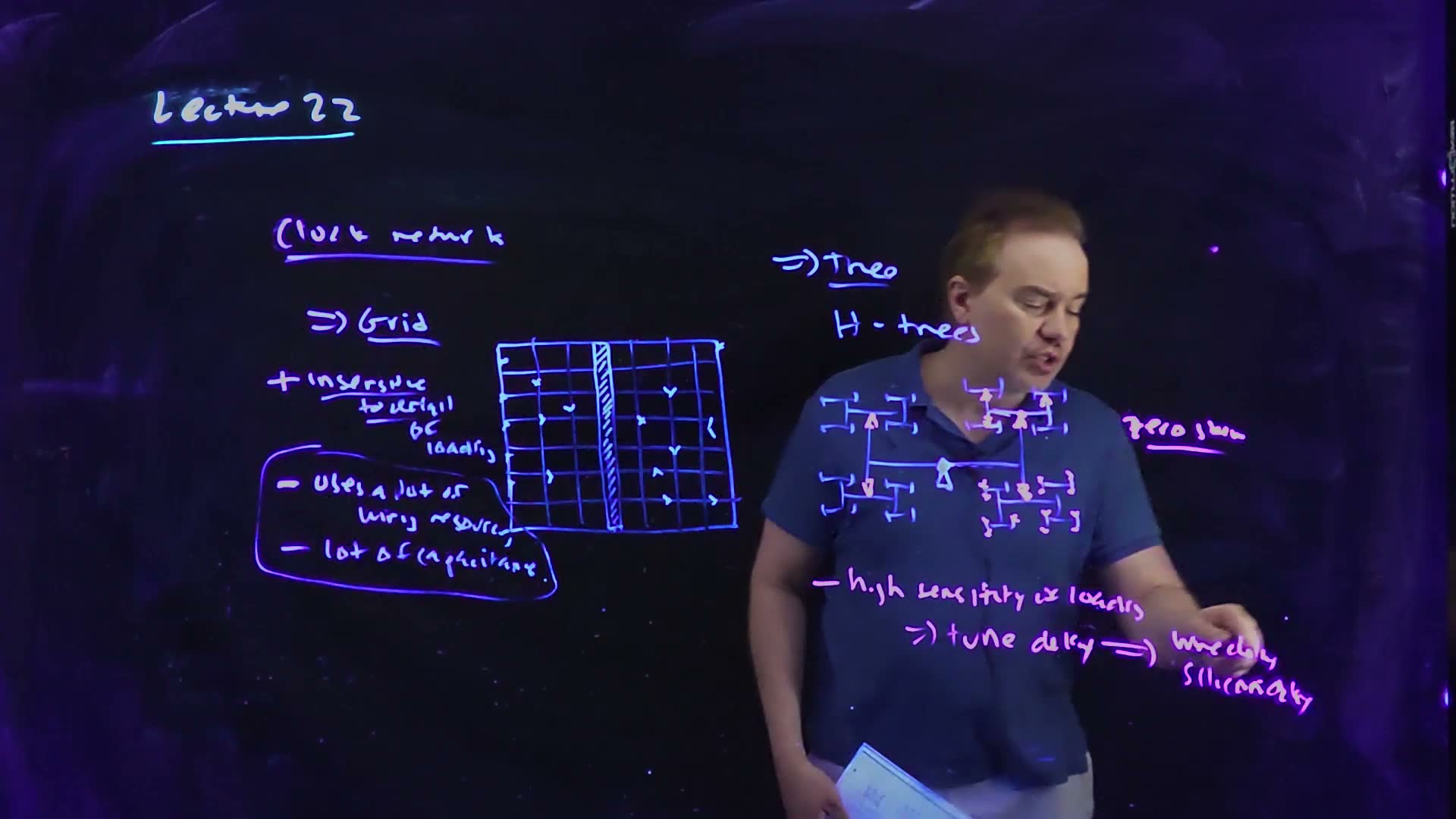
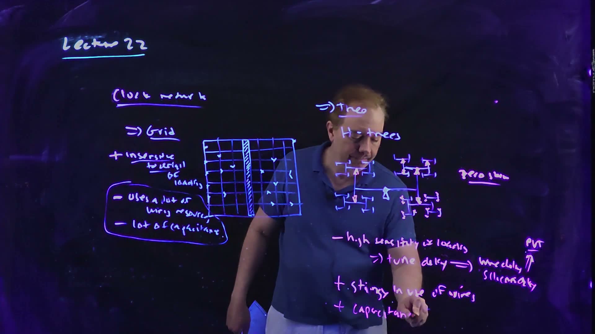
3. Its big minus board (33:52–34:19). High sensitivity to loading. The wires are equal, but the loads at the leaves are not: if one leaf has more flip-flops, its branch is slower. So the tree must be tuned: buffer sizes, wire lengths and widths adjusted until the arrivals match, and retuned after every late change.
4. The tuning rule board (34:33–35:28). “Wire delay and silicon delay have very different … PVT tracking properties … when I tune it, I tune wire for wire, silicon for silicon.” Two branches with equal total delay but a different mix of wire and buffer delay drift apart as soon as the voltage, temperature or process moves.
5. Its pluses board (35:46–36:16). Stingy in its use of wires, and so lower capacitance.
6. The minus is serious (36:16–36:56). Loads change “up until the last minute” of a design, and retuning a tree that is already routed around blockages is hard.

A two-level H-tree board, redrawn (Lecture22 @ 37:14; drawn 32:21–33:40). Buffers sit at the centre of every H. Every path from the root to one of the 16 leaves has the same length: the thick path runs $D/4 + D/4$ on the first H and $D/8 + D/8$ on the second (dimensions added).

The board (Lecture22 @ 37:14)

Lecture22 @ 37:14Trees: the H-tree with distributed buffers, zero skew by geometry; high sensitivity to loading, tuned wire delay against wire delay and silicon against silicon; stingy in wire, lower capacitance.

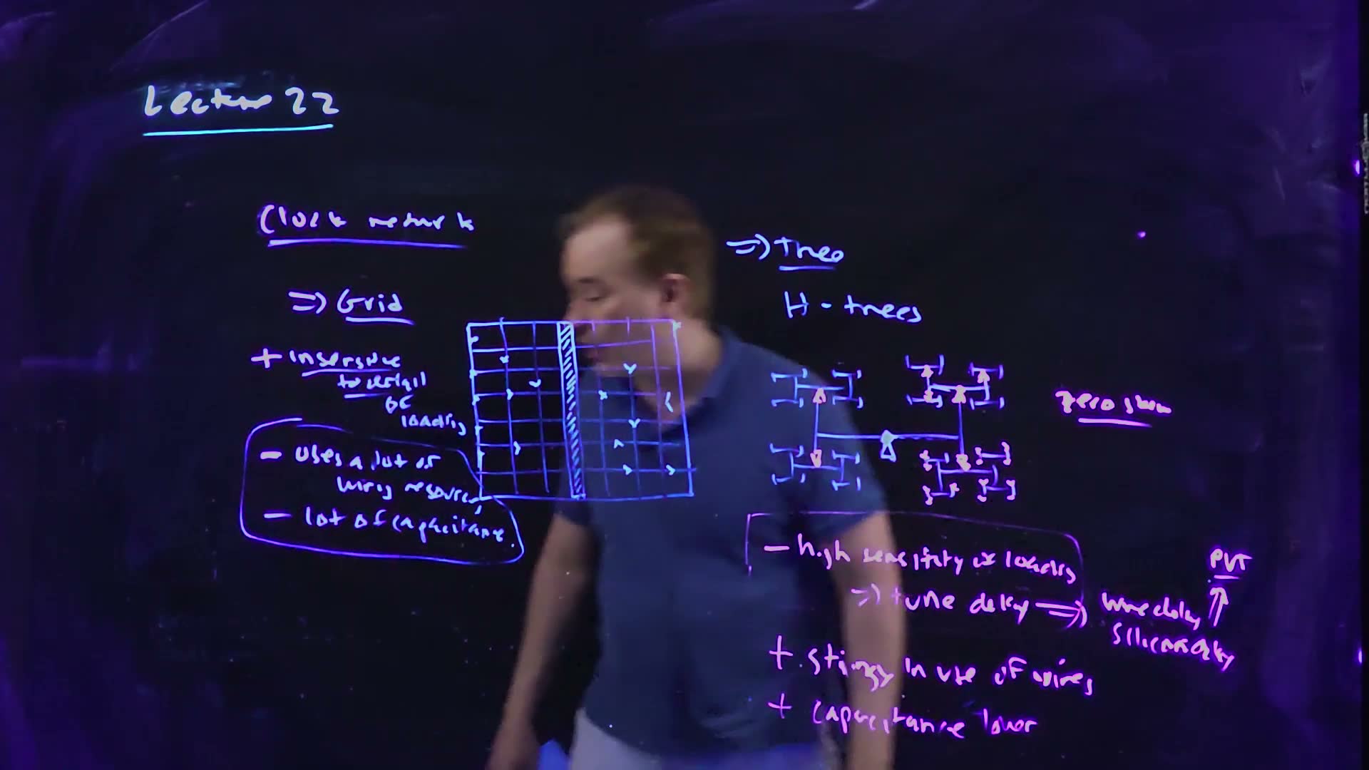
Fair copy of the board above (Lecture22 @ 37:14), mark for mark in its own layout. Black is the pale blue pen: the grid board kept at the left, “Trees”, “H-trees”, the H-tree and its root buffer (the underline of “Lecture 22” is the cyan title pen). Magenta is the pink-violet pen, a second layer: the buffers it drew into the blue tree, drawn here as small filled triangles (one at each second-level node, three in the upper right H and a pair at seven of the lower right H’s eight tips), then “zero skew” and the list of minuses and pluses with its box. The grid’s right half, behind the lecturer’s head, is restored from 31:57; the H-tree’s left half, dimmed by his shirt, is read on 35:49. The buffer chain of 31:57 is wiped by now. The left half repeats the 31:57 copy’s marks one size smaller.

The H-tree’s wire, and the price of a late change

The path and the wire added. Take a square chip of side $D$ and a tree of $k$ levels. The first H spans the chip: its crossbar and its two uprights are each $D/2$ long, $3D/2$ in all, and a path through it runs $D/4$ along the crossbar and $D/4$ up an upright. Each level halves the square, so level $j$ has $4^{j-1}$ H’s of total length $3D/2^j$ each, and a path through level $j$ runs $D/2^j$D/2j. Summing over the levels:

An H-tree's path and wireadded

$$\text{path} = D\left(1 - 2^{-k}\right), \qquad \text{total wire} = \tfrac32\,D\left(2^k - 1\right)$$

Holds when: a square chip of side D, k levels of H's, the root at the centre; 4^k leaves; buffers and the wire widths left out

Derive it from the geometry (two geometric series); it is not worth memorizing.

A worked example: an H-tree against the grid (added; values for example)

1. The same chip. $D$ = 10 mm, and a tree of $k$ = 3 levels: $4^3 =$ 64 leaves.
2. The path. $10 \times (1 - 1/8) =$ 8.75 mm from the root to every leaf.
3. The wire. $1.5 \times 10 \times (8 - 1) =$ 105 mm, against the 1.25 mm grid’s 180 mm (Section 8). At the same 0.2 fF/µm that is 21 pF against 36 pF: the “stingy” tree.
4. A late change. A design change adds 100 fF of flip-flops at one leaf, whose last buffer has a 500 Ω output resistance. That leaf’s clock is later by $R\,\Delta C = 500\ \Omega \times 100\ \text{fF} =$ 50 ps, until the tree is retuned.

Tune wire for wire, silicon for silicon

A worked example: why the mix matters (added; values for example)

1. Two branches, 500 ps each. Branch A: 300 ps of buffer (silicon) delay and 200 ps of wire delay. Branch B: 450 ps of silicon and 50 ps of wire. Nominally the clocks arrive together.
2. A 10 % supply droop. Only silicon slows. With $S_V = -0.4286$ (1.0 V, $V_T$ = 0.3 V), silicon delay grows by $0.4286 \times 0.10 = 4.29$ %. A slows by $0.0429 \times 300 =$ 12.9 ps, B by $0.0429 \times 450 =$ 19.3 ps: 6.4 ps of skew appears.
3. A slow-wire corner. Suppose the wires come out 10 % slower (a high-RC corner) while the transistors are nominal. A slows by 20 ps, B by 5 ps: 15 ps of skew, in the other direction.
4. Matched branches. Tune both to 375 ps of silicon and 125 ps of wire. Under the droop both become 516.1 ps; under the slow wire both become 512.5 ps. The skew stays 0 in both cases.

Why delays are tuned wire for wire and silicon for silicon added, computed with $S_V = -0.4286$−0.4286. (a) Two branches equal in total, 500 ps, but not in kind. (b) A 10 % droop slows only the silicon: 6.4 ps of skew. (c) 10 % slower wire: 15 ps. (d)–(e) Branches matched part for part keep zero skew under both changes.

Check. The droop’s skew is the silicon difference times the fractional change: $(450 - 300) \times 0.0429 = 6.4$ ps; the wire corner’s is the wire difference times 10 %: $(200 - 50) \times 0.1 = 15$ ps.

Traps.

• Balancing a long wire with an extra buffer. It equalizes the nominal delay and leaves the branches mismatched in kind, so they drift apart with every corner.
• “Equal wire length means equal delay.” The loads at the leaves and the buffers along the way must match too; that is the tree’s sensitivity to loading.

Check yourself Why does the tuning rule follow from Chapter 21's remark that only silicon delay depends on V_DD?

A supply change scales only the buffer delays, and a wire corner scales only the wire delays. Two branches with the same silicon delay and the same wire delay change by the same amount under either; two with the same total but a different split change by different amounts, and the difference is skew.

Check yourself Give the same 10 mm chip a four-level H-tree. Find the root-to-leaf path and the total wire, and compare the wire with the grid's.

Path $10 \times (1 - 1/16) =$ 9.375 mm; wire $1.5 \times 10 \times 15 =$ 225 mm, now more than the 1.25 mm grid’s 180 mm. Each level doubles the wire, while the path only approaches $D$D.

Check yourself In the examples, which does the tree more harm: the late 100 fF load or the 10 % droop on unmatched branches?

The late load: 50 ps of skew, against 6.4 ps from the droop. A load change acts on the whole RC of one branch at once, while the droop acts only on the silicon difference between branches. That is why the H-tree’s minus is its “sensitivity to loading”.

10. Tree-driven grids

You need

The grid (Section 8): a low-resistance mesh, insensitive to where the loads are, but heavy in wire and capacitance.

The clock grid (Section 8). Original figure ↑

The H-tree (Section 9): equal paths to every leaf and little wire, but sensitive to the loads at the leaves, so it must be tuned and retuned.

The two-level H-tree (Section 9). Original figure ↑

The question. Each pure network has one serious minus. “Is there a way I can combine these two?” (36:56)

The tree-driven grid (board, 36:56–39:39)

1. Where things have wound up (36:56–37:23). As the lecturer told it at the recording, both Intel and IBM use tree-driven grids, and Intel adds deskewing (Section 7).
2. The structure board (37:42–38:48). A tree delivers the clock, with equal paths, to many taps spread over a grid. Because the grid is driven at many points, it can be much lighter than a pure grid.
3. Why it works (38:48–39:09). The grid shorts the taps together and averages out the “loading inhomogeneities”: a load added late, between taps, is shared by the taps around it, so the tree need not be retuned.

A tree-driven grid board, redrawn (Lecture22 @ 39:39; begun at 38:36). A two-level H-tree delivers the clock to 16 taps (dots) on a lighter grid, which shorts the taps together. The board draws two of the tap dots; all 16 are drawn here. The grid is drawn with 8 × 8 cells so that the taps fall on its nodes (the board’s has about 7 × 5).

The board (Lecture22 @ 39:39)

Lecture22 @ 39:39The tree-driven grid: a tree feeding a grid at many taps.

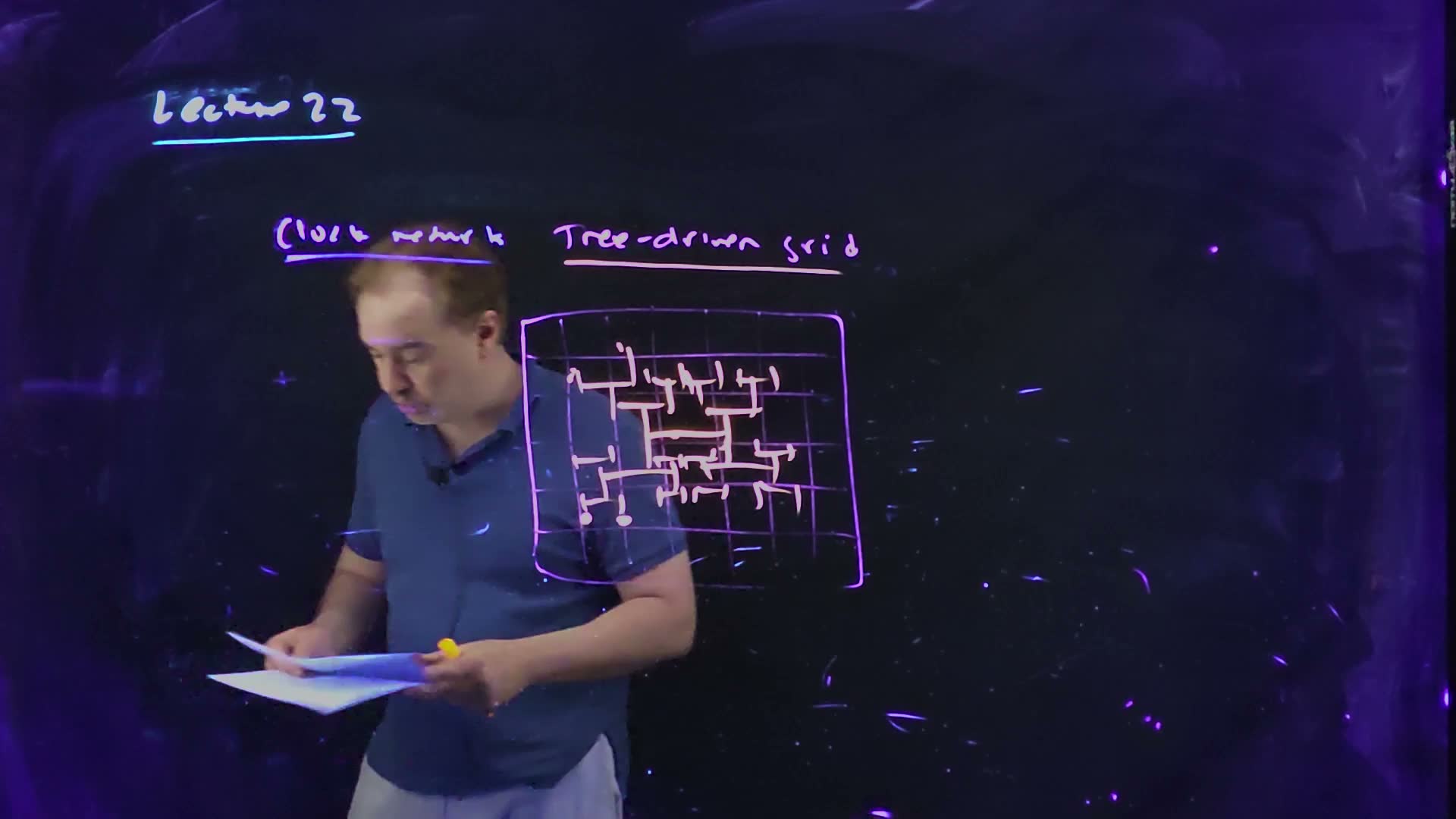
Fair copy of the board above (Lecture22 @ 39:39), mark for mark in its own layout. Black is the violet pen: the rounded rectangle, the grid (seven columns, six rows) and “Tree-driven grid”; “Clock network” (pale blue) and “Lecture 22” (its underline the cyan title pen) are kept from the earlier boards. Orange is a pale pink-white pen, a second layer: the tree drawn over the grid, its two tap dots and the underline of “Tree-driven grid”. The tree is copied stroke by stroke as the hand drew it, nested H’s with short ticks at their tips, not tidied into a regular H-tree. Nothing is hidden: the lecturer stands behind the strokes (the grid checked on 38:36). The grid’s second line from the top starts only at its middle, as on the board.

A worked example: a lighter grid (added; values for example, from Sections 8–9)

1. The tree. On the same 10 mm chip, a two-level H-tree reaches $4^2 =$ 16 taps with $1.5 \times 10 \times 3 =$ 45 mm of wire. The taps sit at the centres of a 4 × 4 array of 2.5 mm squares.
2. The grid. Run a grid line through each row and each column of taps: 4 lines each way, 10 mm long, pitch 2.5 mm: 80 mm of wire.
3. The total. $45 + 80 =$ 125 mm: more than the 105 mm three-level tree, but well under the pure 1.25 mm grid’s 180 mm.
4. How far from a tap. Along any grid line the taps are 2.5 mm apart and the outermost taps sit 1.25 mm from the edge, so no point of the grid is more than 1.25 mm of wire from a tap. A late load anywhere is close to a driven point and shares its charge with the taps around it.

Traps.

• “The grid removes the need for a balanced tree.” The taps must still receive their clock together; the grid only absorbs the differences the loads make between them.

Check yourself Which minus of each pure network does the tree-driven grid keep, and which does it drop?

From the grid it drops most of the wire and capacitance, because the grid is driven at many points and can be sparse; it keeps a little of both (the 80 mm of grid in the example). From the tree it drops the sensitivity to loading, because the grid averages the loads between taps; it keeps the need to balance the tree itself to the taps.

11. Energy-constrained design and wasted power

You need

Two kinds of power (Chapter 6). Switching a node of capacitance $C$ at frequency $f$ costs $CV_{DD}^2f$ (dynamic power). In either state, one transistor of a static gate is off with $V_{DD}$ across it and leaks a current $I_{leak}$Ileak​, which costs $V_{DD}I_{leak}$ all the time (leakage power).

Why power became the limit (Chapter 4). Under Dennard scaling the supply fell with the dimensions and power density stayed constant. The threshold could not keep falling without leakage exploding (tenfold per subthreshold slope $S$S, about 60–100 mV), so the supply stopped scaling, and power density rose with every generation.

The question. Once the supply stopped scaling, a chip’s power became a hard limit. What sets the limit, and where does the first, easiest saving come from?

Power as a constraint (board, 40:18–44:43)

1. The name board (40:18). “Low-power design”, which the lecturer calls better named energy-constrained design: the goal is not to be slow, but to do each operation with as little energy as the power budget demands.
2. What changed (40:32–41:34). Power used to be whatever the design came out at. When supplies stopped scaling, power density and chip power rose, and now packaging sets the limit: how much heat the package and the cooling can carry away.
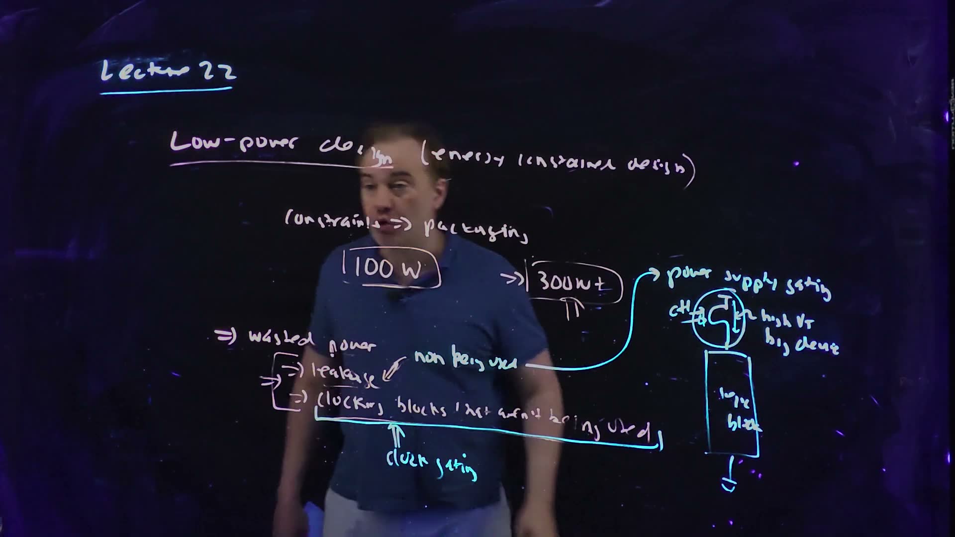
3. The numbers board (41:34–41:51). The lecturer’s “Dell’s law”: spend no more than $25 on packaging and power supply, which puts a desktop processor at about 100 W. Mainframes, with expensive packaging and cooling, go to 300 W and up.
4. Useful and wasted power board (42:49–43:30). Some power does useful work; some is wasted. The wasted power has two sources: leakage of blocks that are not being used, and clocking blocks that aren’t being used.
5. The lowest hanging fruit (43:38–44:09). Removing wasted power costs no performance, so it comes first: every processor does it (Section 12).
6. Leakage in an active block (44:09–44:43). In a block that is working, leakage cannot be avoided: in an optimal design it is, the lecturer says, about 30 % of the block’s power. (Said, not derived. Section 16 finds a different share in a different optimization.)

Where power is wasted added, after the board’s list (Lecture22 @ 47:42). Two blocks are working (shaded) and two are idle. An idle block still leaks ($I_{leak}$Ileak​ from $V_{DD}$VDD​), and if its clock still toggles (clk), it still charges its clock load every cycle. The AND gate at each block’s clock input is where clock gating acts (Section 12).

A worked example: a power budget (added; values for example)

1. The budget. A 100 W processor at 1.0 V.
2. An active block. Its switching power is 7 W. If leakage is 30 % of its total, as the lecture says of an optimal block, the total is $7/0.7 =$ 10 W and the leakage 3 W. That leakage is the price of a fast block, not waste.
3. An idle copy. A second copy of the block with nothing to do still leaks its 3 W, and if its clock keeps running it also burns its clock power, every cycle. Both are waste, and both can be removed (Section 12).

Traps.

• “Low-power means slow.” The constraint is energy per operation inside a power budget; the design is still as fast as the budget allows.
• “All leakage is waste.” Leakage in a block that is working is the cost of its speed; only the leakage of idle blocks is wasted.

Check yourself Why does leakage in an idle block count as wasted, while leakage in an active block does not?

An active block’s leakage comes with the low threshold that makes it fast; removing it would cost speed. An idle block does no work at all, so any power it draws, leakage or clocking, buys nothing, and turning it off costs nothing but the time to turn it back on.

Check yourself Why does packaging, not the transistors, set a desktop processor's power near 100 W?

The transistors would happily burn more. What limits a chip’s power is how much heat can be carried away and at what cost: the package, the heat sink and the power supply. The lecturer’s “Dell’s law” caps that cost, and with it the power; a mainframe, which can afford more cooling, goes past 300 W.

12. Power gating and clock gating

You need

Leakage and the threshold (Chapter 4). Below threshold a transistor’s current falls tenfold for every $S$ of gate voltage, where $S$ is the subthreshold slope (60 mV/decade at best, 80–100 in real devices). A device’s off current scales as $10^{-V_T/S}$10−VT​/S, so raising $V_T$ by $\Delta V_T$ cuts its leakage by $10^{\Delta V_T/S}$10ΔVT​/S.

On-resistance (Chapter 7). A transistor’s on-resistance falls as its width grows: $R = R_{unit}/W$Runit​/W, with $R_{unit}$ in kΩ·µm.

Local clock generators (Chapter 14). The global clock is one wire; near the flip-flops, local generators make the phases the latches need ($\phi_1$ϕ1​, $\phi_2$ϕ2​).

Clock power (Section 8): $P = C_{clk}V_{DD}^2 f$Cclk​VDD2​f.

The question. Section 11 named two wastes: an idle block’s leakage and an idle block’s clock. How is each switched off, and what does each switch cost?

Two kinds of gating (board, 44:50–47:42)

1. Power-supply gating board (45:06–45:23). Put a switch between $V_{DD}$ and the logic block, driven by a control signal (the board’s “ctl”). When the block is idle, open the switch: the block’s supply collapses and it stops leaking.
2. What kind of switch board (45:23–45:48). A high-$V_T$ device, so that the switch itself leaks little when it is off; and a big device, so that it drops little voltage when it is on and the block’s speed does not suffer. Its large gate capacitance does not matter, because it is switched rarely: “not doing this very often”.
3. Where the clock ends (46:20–46:51). Clock distribution ends at local clock generators, which make $\phi_1$ and $\phi_2$ from the single-wire global clock.
4. Clock gating board (46:51–47:22). In the local generator, AND the clock with a gate signal. With gate = 0 the local clock stops: nothing is launched, no logic evaluates, and the clock load stops switching.

Gating board, redrawn (Lecture22 @ 47:42). (a) Power-supply gating: a high-threshold, wide PFET header (the board’s “high V_T, big device”), driven by ctl, between $V_{DD}$ and the logic block; the node below it is the block’s virtual supply $V_{DD,v}$ (label added). (b) Clock gating: clk AND gate drives the local clock generator, which makes $\phi_1$ and $\phi_2$ (added, from 46:20).

The board (Lecture22 @ 47:42)

Lecture22 @ 47:42Energy-constrained design: packaging sets the budget (100 W, 300 W+); wasted power is leakage and clocking of idle blocks, removed by power-supply gating and clock gating.

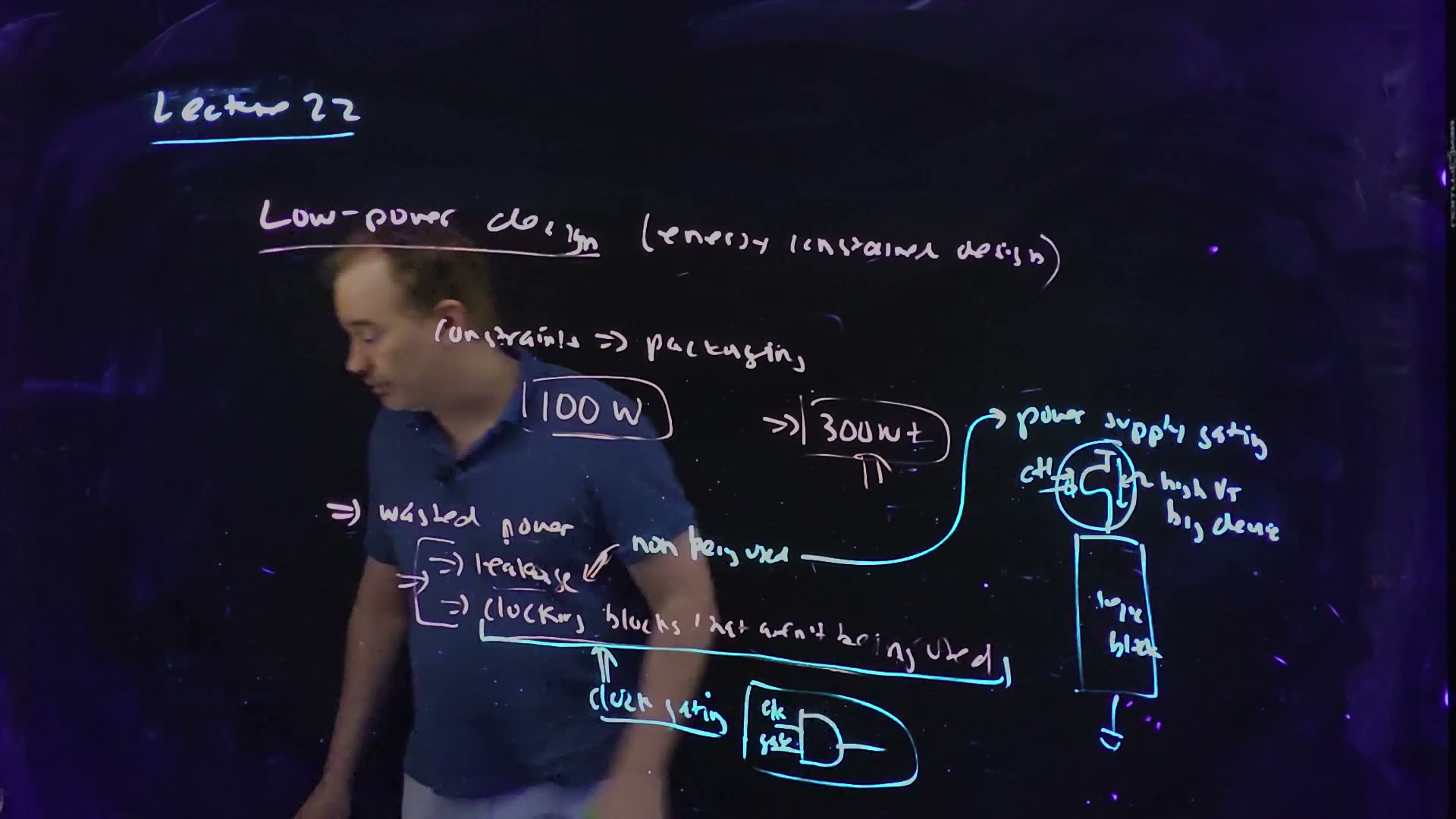
Fair copy of the board above (Lecture22 @ 47:42), mark for mark in its own layout. Black is a pale pink-white pen: the text from “Low-power design” down to the list of wasted power, “non being used” with its arrow to “leakage”, and a first underline under “clocking blocks that aren’t being used” (“Lecture 22“‘s underline is the cyan title pen). Teal is the cyan pen, a second layer: the remedies, drawn from 44:57 on. They are the long arrow from “non being used” to “power supply gating”; the ringed header PFET with “ctl”, “high V_T” and “big device”, the logic block and its ground; and the cyan underline traced over the pale one, its double arrow, “clock gating” and the ringed AND of clk and gate. † “non” is the board’s slip for “not”: the speech says “a block that’s not being used” (44:43–44:50). There the hand runs the i and n of “being” together; it is set as “being”. Nothing is hidden: the lecturer stands behind the strokes (the list checked on 45:18 and 46:23). Where the typeset words run wider than the hand’s they are spread a little, and the AND gate sits slightly right of the board’s to clear its labels.

Sizing the gatesadded

$$R_{on} \le \frac{\Delta V_{allowed}}{I_{block}}, \qquad W \ge \frac{R_{unit}}{R_{on}}$$$$\frac{I_{leak}(V_T)}{I_{leak}(V_T + \Delta V_T)} = 10^{\Delta V_T/S}$$$$P_{saved} = (\text{idle fraction})\,C_{clk}V_{DD}^2 f$$

Holds when: a header switch carrying the block's whole current I_block with an allowed drop ΔV; R_unit the switch device's resistance-width product; leakage below threshold with slope S; a clock gated for a fraction of the time

Derive each: Ohm’s law for the header; the subthreshold line for the leakage; $CV^2f$ for the clock.

A worked example: sizing a header and gating a clock (added; values for example)

1. The block. For example, it draws 100 mA at 1.0 V, and the header may drop 2 % of the supply, 20 mV.
2. The header’s resistance. $R_{on} \le 0.020/0.100 =$ 0.20 Ω.
3. Its width. With a high-$V_T$ PFET of 2 kΩ·µm (illustrative), $W \ge 2000/0.20 =$ 10,000 µm: a centimetre of transistor width, “a very big device”.
4. Its own leakage. At $S$ = 90 mV/decade, a threshold 100 mV higher than the logic’s cuts the switch’s leakage by $10^{100/90} =$ 12.9 times; 150 mV higher, by 46.4 times.
5. Clock gating. The block’s clock load is 200 pF; at 1 V and 2 GHz it burns $200\ \text{pF} \times 1 \times 2\ \text{GHz} =$ 0.40 W. If the block is idle 70 % of the time, gating its clock saves $0.7 \times 0.40 =$ 0.28 W.

Check. The header’s drop at full current is $0.20\ \Omega \times 100\ \text{mA} = 20$ mV, the allowed 2 %; a header half as wide would drop 40 mV and slow the whole block.

Traps.

• A low-$V_T$ switch. It would leak almost as much as the block it is meant to turn off.
• A small switch. Its IR drop lowers the block’s supply, and Section 6’s sensitivity turns that into delay.
• A glitchy gate signal. If gate changes while clk is high, the AND passes a truncated pulse. The gate signal must change only while clk is low added (the same care as Chapter 14’s clock chopper).

Check yourself Why may the header's gate be slow?

The block is put to sleep and woken rarely, on a scale of microseconds or more, so the header’s huge gate capacitance is charged rarely too; its energy and its delay are paid once per sleep, not once per cycle.

Check yourself The block draws 250 mA and may drop only 1 % of 1.0 V. Find R_on and the header width at 2 kΩ·µm.

$R_{on} \le 0.010/0.250 =$ 0.04 Ω; $W \ge 2000/0.04 =$ 50,000 µm, 5 cm of width: five times the example’s, because the current is 2.5 times larger and the allowed drop half as big.

Check yourself Which gating saves leakage, and which saves dynamic power?

Power-supply gating removes the idle block’s leakage (and, with its supply gone, everything else it draws). Clock gating removes the idle block’s dynamic power: its clock load and the logic the clock would have made switch. Clock gating does nothing for leakage, because the block is still powered.

13. The energy–delay curve: V_DD as the knob

You need

Switching energy (Chapter 6). Each time a node of capacitance $C$ rises, the supply delivers $CV_{DD}^2$ (half stored on $C$C, half lost in the PFET). So the dynamic energy per operation goes as $V_{DD}^2$VDD2​. Leakage power is $V_{DD}I_{leak}$VDD​Ileak​, linear in $V_{DD}$ at a fixed leakage current.

The supply and the delay (Chapter 5). A gate’s delay is about the charge it moves over the current that moves it, $t \propto CV_{DD}/I$CVDD​/I. With the velocity-saturated current $I \propto V_{DD} - V_T$VT​, $t \propto V_{DD}/(V_{DD} - V_T)$VT​): the delay rises as $V_{DD}$ falls, without limit as $V_{DD}$ approaches $V_T$VT​.

The question. A design can be made faster by spending more energy, or frugal by accepting more delay. What does the set of the best possible designs look like, and which knob moves a design along it?

The energy–delay curve (board, 48:13–52:32)

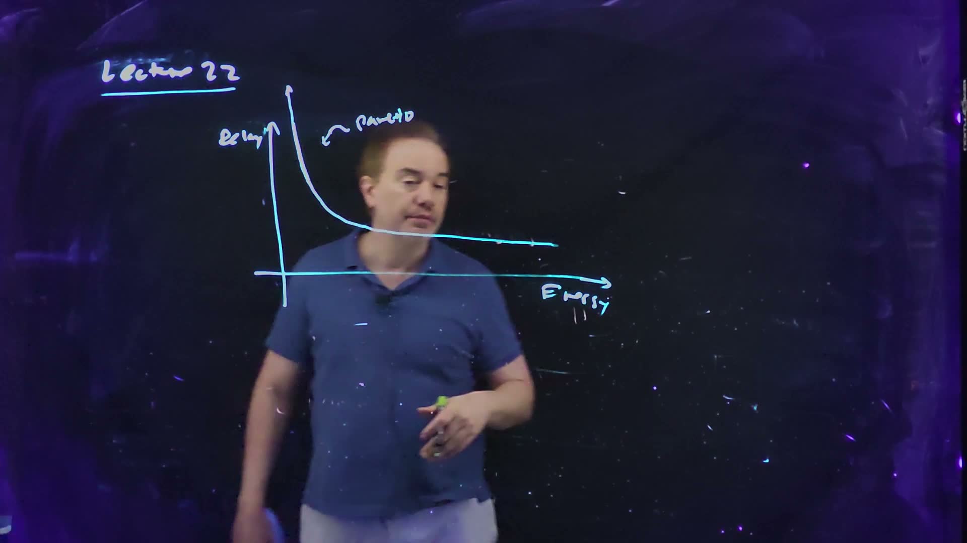
1. The axes board (48:13–48:48). Delay on the vertical axis, energy (per operation) on the horizontal one. A task done with little energy takes a long time; done quickly, it takes a lot of energy.
2. The Pareto curve board (49:18). The best designs achievable trace a curve: a Pareto curve. No design lies below and to the left of it, and a design above and to the right of it wastes energy or time.
3. Two regions of diminishing returns board (49:18–49:51). Near the delay axis the curve is steep: a little less energy costs a lot of delay. Near the energy axis it is flat: a little more speed costs a lot of energy.
4. How to use it (49:51–51:00). Know the workload’s deadline, sit on the curve at that delay, and burn no more energy than that point needs. Never sit off the curve.
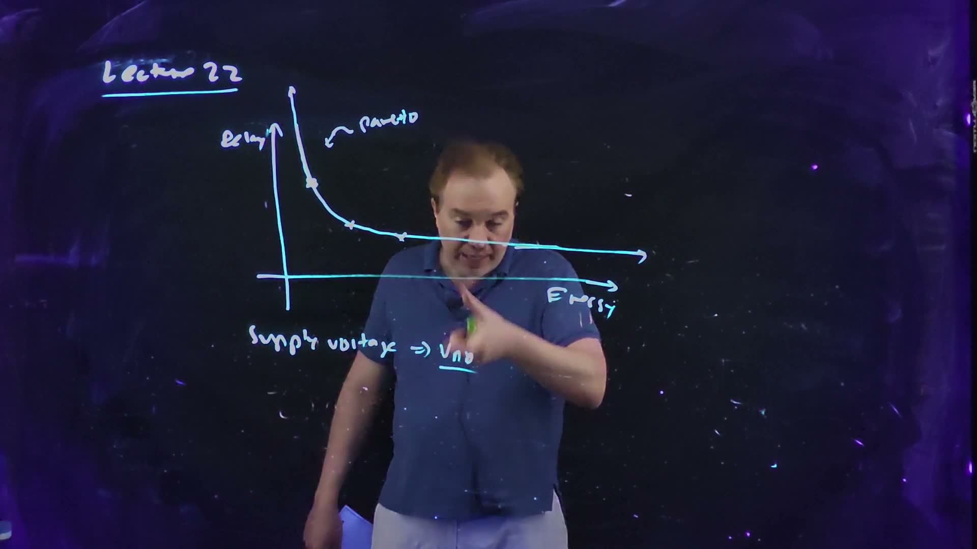
5. The knob board (51:24–51:36). “The best knob that you have to play with is the supply voltage”: “I will save dynamic power as $V_{DD}$ squared, I’ll save leakage power linearly with $V_{DD}$VDD​”, and the delay rises.
6. Parallelism (52:00–52:32). Two units, each at half speed, finish the same work in the same time. Half speed allows a lower supply, so each operation costs less energy: same throughput, less power.

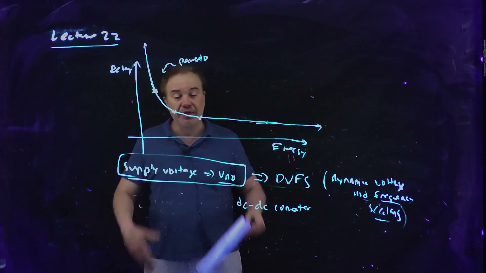
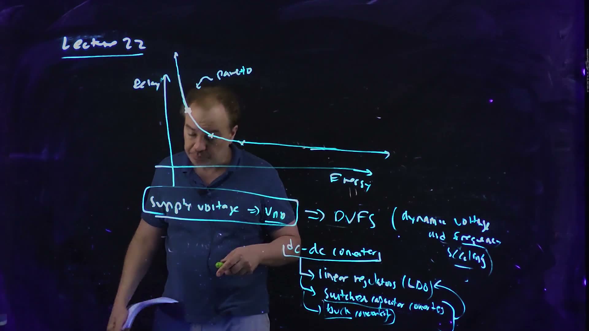
The energy–delay curve board, redrawn (Lecture22 @ 57:49; built 48:38–52:10). Delay $t$ up, energy $E$ across; the best designs lie on this Pareto curve, with diminishing returns at both ends. The supply voltage moves a design along it (the board’s “supply voltage ⇒ V_DD”, then DVFS). The ring marks the low-energy, long-delay end, where the board writes “subthreshold” (Sections 15–16).

The board (Lecture22 @ 57:49)

Lecture22 @ 57:49The energy–delay Pareto curve; the supply voltage as the knob; DVFS and the three kinds of dc–dc converter; the ring at the subthreshold end.

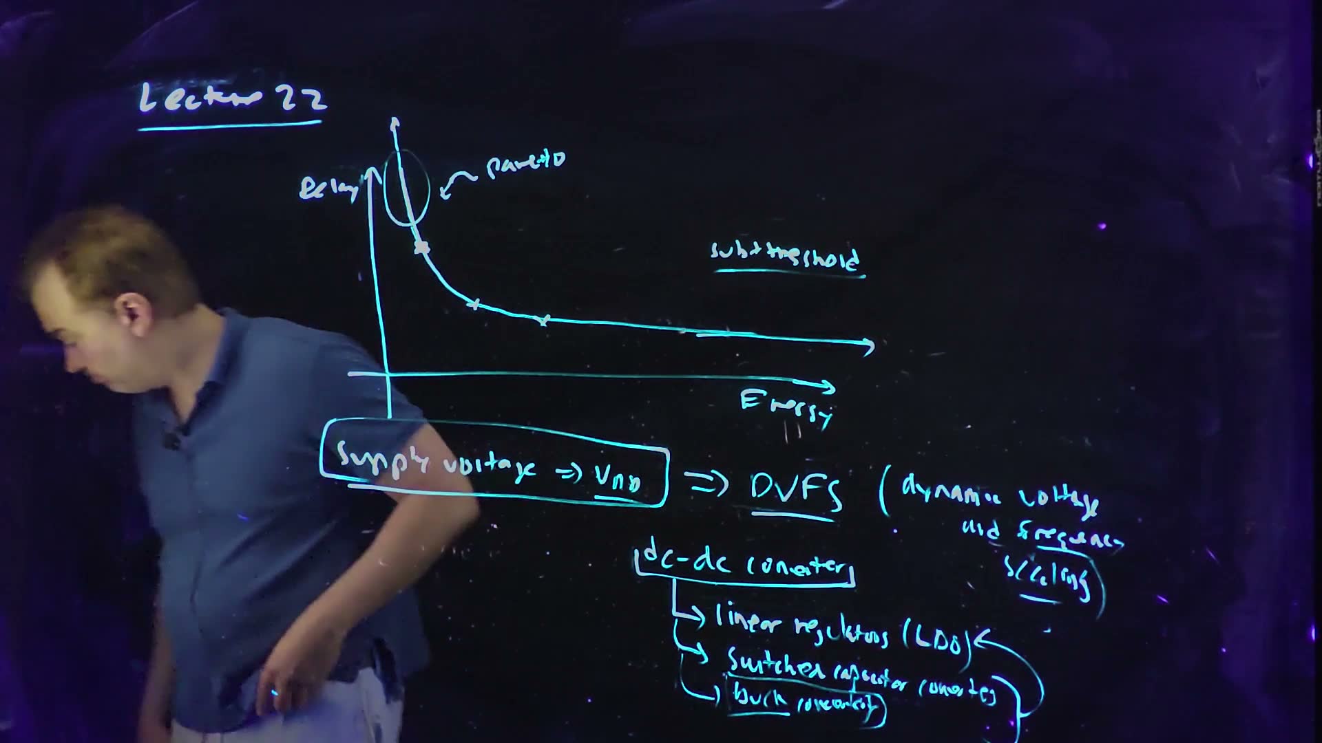
Fair copy of the board above (Lecture22 @ 57:49), mark for mark in its own layout, all in black: one cyan pen wrote the whole board. Nothing is hidden: the lecturer stands behind the strokes (the axes and the curve checked on 52:10). The curve’s right end is traced twice for a short stretch, and both strokes are copied. The hand writes the two D’s of V_DD as open loops that read like “nn”. A faint pale double stroke under “Energy”, left from the erased 47:42 board, is left out. Where the typeset words run wider than the hand’s, “capacitor converters” and the buck’s “converters” are set smaller, and the stroke beside the converters and the foot of the return arrow sit a little right of the board’s.

The curve from the course’s models

Energy and delay against the supplyadded

$$\frac{E}{E_0} = \left(\frac{V_{DD}}{V_0}\right)^2, \qquad \frac{t}{t_0} = \frac{V_{DD}/(V_{DD} - V_T)}{V_0/(V_0 - V_T)}$$$$\frac{t}{t_0} = r \;\Longleftarrow\; V_{DD} = \frac{\rho\,V_T}{\rho - 1},\quad \rho = \frac{r\,V_0}{V_0 - V_T}$$

Holds when: dynamic energy only (leakage left out); a velocity-saturated device above threshold, V_DD > V_T; relative to a nominal supply V₀; the same circuit at every supply

Memorize the first two (from Chapters 5–6). Derive the third: set $V/(V - V_T) = \rho$ and solve for $V$V.

A worked example: moving along the curve (added; V_T = 0.3 V, nominal 1.0 V, for example)

1. Up the supply, to 1.2 V. Delay $\times$0.933, energy $\times$1.44: 7 % faster for 44 % more energy, the flat end.
2. Down to 0.6 V. Delay $\times$1.40, energy $\times$0.36.
3. Down to 0.4 V. Delay $\times$2.80, energy $\times$0.16: now each further saving costs a lot of delay, the steep end.
4. Half speed. For $t/t_0 = 2$2: $\rho = 2 \times 1.0/0.7 = 2.857$2.857, so $V = 2.857 \times 0.3/1.857 =$ 0.4615 V. The energy per operation is $0.4615^2 =$ 0.213 of nominal: a 79 % saving for twice the delay.
5. Two cores at half speed. Together they give the original throughput, each operation at 0.213 of the energy: 0.213 of the dynamic power. Their leakage is another matter: each leaks at 0.4615 of the nominal voltage, but there are two, so 0.923 of one core’s leakage power.

The energy–delay curve computed from the course’s models added: $E/E_0 = V^2$ and $t/t_0 = [V/(V - 0.3)]/[1/0.7]$ ($V_T$VT​ = 0.3 V, nominal 1.0 V), points labelled with $V_{DD}$VDD​. The hollow point is half speed, 0.4615 V, at 0.213 of the energy. The dashed line is the delay floor, 0.7, as $V_{DD}$ grows without bound; the steep end climbs without bound as $V_{DD}$ approaches $V_T$ in this model, and below threshold Sections 15–16 take over.

Check. The half-speed supply satisfies the delay ratio: $0.4615/(0.4615 - 0.3) = 2.857$2.857, twice $1.0/0.7 = 1.429$1.429.

Traps.

• “Energy falls in proportion to speed.” It falls as $V^2$ while the delay rises as $V/(V - V_T)$VT​): slow by 2 for a factor of 4.7 in energy here, then much less per step near $V_T$VT​.
• Leakage energy per operation. Leakage power falls linearly with $V_{DD}$VDD​, but each operation takes longer, so the leakage energy per operation, power times time, falls more slowly and can even rise. Section 16 makes this the limit.

Check yourself Which end of the curve does a phone in standby want, and which a server in a burst of requests?

The phone in standby has no deadline worth the name: it wants the steep, low-energy end (low $V_{DD}$VDD​, long delay). The server in a burst must meet latency targets: it moves toward the flat end, buying speed with energy.

Check yourself For 70 % of the nominal speed, find the supply and the energy per operation (V_T = 0.3 V, nominal 1.0 V).

70 % of the speed is $1/0.7 = 1.4286$ times the delay. $\rho = 1.4286 \times 1.0/0.7 = 2.041$2.041, so $V = 2.041 \times 0.3/1.041 =$ 0.588 V, and the energy is $0.588^2 =$ 0.346 of nominal: 65 % saved for 30 % less speed.

14. DVFS and on-chip dc–dc converters

You need

The knob (Section 13). Lowering $V_{DD}$ cuts the switching energy per operation as $V_{DD}^2$ and slows the gates as $V_{DD}/(V_{DD} - V_T)$VT​).

The computed energy–delay curve (Section 13). Original figure ↑

Dynamic power (Chapter 6). Energy per operation times operations per second: $P = \alpha C V_{DD}^2 f$αCVDD2​f, with $\alpha$ the fraction of the capacitance $C$ that rises each cycle, so power scales as $V_{DD}^2 f$ for a given circuit.

The question. A chip’s workload changes from moment to moment. How does it move along the energy–delay curve at run time, and where does the variable supply come from?

DVFS and its converters (board, 52:58–55:40)

1. DVFS board (52:58). Dynamic voltage and frequency scaling: set the supply and the clock frequency together, at run time, to suit the workload. A heavy workload raises $V_{DD}$ and $f$f; a light one lowers both.
2. The converter board (53:17–53:59). The variable supply comes from a dc–dc converter on the chip, which steps down from the highest supply the chip receives.
3. Three kinds board (54:20–55:13), named only: linear regulators (LDO, low dropout); switched-capacitor converters; and buck converters, which use inductors and reach a higher efficiency but are harder to integrate. “We’re not going to talk about these” in detail. (The lecturer’s start-up made on-chip magnetic inductors for such converters.)
4. The principle of each added. An LDO is a transistor whose resistance a feedback loop adjusts so that it drops exactly $V_{in} - V_{out}$Vout​; the current through it is the load’s, so its efficiency is at most $V_{out}/V_{in}$Vout​/Vin​. A switched-capacitor converter shuffles charge between capacitors in two phases, giving fixed ratios such as 2:1 efficiently. A buck converter switches a node between $V_{in}$ and ground and filters it with an inductor and a capacitor; the inductor moves energy without dropping a voltage across a resistance.
5. The order (55:13–55:40). First remove the wasted power (Section 12); then trade energy against delay with DVFS.

Three on-chip dc–dc converters added, after the board’s list (Lecture22 @ 57:49). (a) A linear regulator (LDO): a pass transistor in a feedback loop. (b) A 2:1 switched-capacitor converter, its switches on two phases. (c) A buck converter: a switched node $V_x$ filtered by $L$ and $C$C.

A worked example: DVFS with an LDO (added; values for example, from Section 13)

1. The setting. The workload needs only 0.7 of the nominal clock frequency. At 0.6 V the gates are 1.40 times slower (Section 13), so they can still run at $1/1.40 = 0.714$ of the frequency: 0.6 V and 0.7 $f$ is a valid setting.
2. The core’s power. $(0.6)^2 \times 0.7 =$ 0.252 of its nominal dynamic power.
3. The converter’s cost. An LDO from a 1.0 V input to 0.6 V passes the core’s current and drops 0.4 V across itself: its efficiency is at most $0.6/1.0 =$ 60 %, so at least 40 % of the power drawn from the input is lost.
4. Still a saving. Drawn from the 1.0 V input, the core costs at least $0.252/0.6 =$ 0.42 of its nominal power. An efficient buck converter would bring that close to 0.252.

Traps.

• Frequency without voltage. Lowering $f$ alone lowers the power, but each operation still costs $CV_{DD}^2$CVDD2​: the energy per operation, and so the battery’s work per task, is unchanged.
• A setting the gates cannot meet. The frequency must stay below what the gates allow at the chosen supply.

Check yourself When the workload is light, why lower V_DD and not only f?

Lowering $f$ alone stretches the same energy per operation over more time: power falls, energy per task does not. Lowering $V_{DD}$ as well (as far as the slower frequency allows) cuts each operation’s energy as $V_{DD}^2$VDD2​; that is what saves the battery.

Check yourself At 0.8 V and 0.85 of the frequency, what is the core's dynamic power relative to 1.0 V and full frequency? Is the setting valid (V_T = 0.3 V)?

$0.8^2 \times 0.85 =$ 0.544. At 0.8 V the delay is $[0.8/0.5]/[1/0.7] = 1.12$ times nominal, so the gates allow $1/1.12 = 0.893$ of the frequency: 0.85 is within it, so yes.

15. How low can V_DD go? The functional limit

You need

Subthreshold current (Chapter 4; FN2’s conventions). Below threshold, a transistor’s current grows tenfold for every $S$ of gate voltage, where $S$ is the subthreshold slope (60 mV/decade at best, 80–100 in real devices):

$$I = I_{off}\,10^{V_{GS}/S},$$

with $I_{off}$ the current at $V_{GS} = 0$0. If both “on” ($V_{GS} = V_{DD}$VGS​=VDD​) and “off” ($V_{GS} = 0$VGS​=0) are below threshold, $I_{on}/I_{off} = 10^{V_{DD}/S}$10VDD​/S. This line has no drain voltage in it: it assumes $V_{DS}$ is large.

Where the lecture stops (55:44–56:43). Supplies now often sit “just barely above the threshold voltage”, and below $V_T$VT​, subthreshold operation is possible. The board rings the low-energy end of the energy–delay curve.

The energy–delay curve, with the subthreshold end ringed (Section 13). Original figure ↑

The question. added Below threshold an inverter still switches: it is just slow. But its “on” transistor is only $10^{V_{DD}/S}$ times stronger than its “off” one, a few times rather than a million. As $V_{DD}$ falls, the off device’s leakage pulls the low output up toward the middle. How low can the supply go before the output no longer reaches a valid 0? This is FN10-2c’s question.

The low output of a subthreshold inverter (added)

1. Swiss watches (55:44–56:55). Operating just above $V_T$ is common; below it is possible, and “the Swiss have done this in watches”.
2. The setting. The input is high, so the NFET is on and pulls the output down, while the PFET is off but leaks current into the output. The output settles where the two currents are equal. Above threshold the NFET wins by orders of magnitude and the output sits at 0. Below threshold it wins only by a small factor.
3. Why the course’s line is not enough. In $I = I_{off}10^{V_{GS}/S}$ the current does not depend on $V_{DS}$VDS​. Then the NFET’s current would be larger than the PFET’s at every output voltage, even with the output at 0 V and nothing across the NFET, and no balance point would exist. A transistor with no voltage across it carries no current, so the line must be missing a factor that vanishes as $V_{DS} \to 0$0.
4. The drain factor (background device physics). Below threshold the current is carriers diffusing over a barrier at the source end of the channel. Carriers also diffuse back over the barrier at the drain end, which is higher by $qV_{DS}$qVDS​, so the back-flow is smaller by $e^{-V_{DS}/(kT/q)}$e−VDS​/(kT/q). The net current is $I = I_0\,10^{V_{GS}/S}\left(1 - e^{-V_{DS}/(kT/q)}\right),$ where $kT/q$ = 26 mV is the thermal voltage. The factor uses $kT/q$kT/q, not $S$S: the drain sets the barrier directly, not through the gate’s imperfect coupling. For $V_{DS}$ above about $3kT/q$ = 78 mV the factor exceeds 0.95, which is why Chapter 4 and FN2 could leave it out. Near a low output, though, the NFET’s $V_{DS}$ is a few millivolts, and the factor is what lets the output settle.
5. The balance. Take the input from an identical stage, so a “high” input is itself only $0.9V_{DD}$ at the limit. The NFET has $V_{GS} = 0.9V_{DD}$ and $V_{DS} = V_{out}$Vout​; the PFET has $V_{SG} = V_{DD} - 0.9V_{DD} = 0.1V_{DD}$ and $V_{SD} = V_{DD} - V_{out}$Vout​. With matched devices the $I_0$ cancels: $10^{0.9V_{DD}/S}\left(1 - e^{-V_{out}/(kT/q)}\right) = 10^{0.1V_{DD}/S}\left(1 - e^{-(V_{DD} - V_{out})/(kT/q)}\right).$ The left side rises from 0 with $V_{out}$Vout​; the right side falls to 0; they cross once.
6. The limit. Call a low output valid if it is at most $0.1V_{DD}$0.1VDD​. Set $V_{out} = 0.1V_{DD}$ and solve for $V_{DD}$VDD​: that supply is the functional limit $V_{fn}$Vfn​. The equation has no closed form; try values of $V_{DD}$ (or iterate) until the two sides agree.
7. Simplifications an exam may accept; say which you use. (a) Drop the PFET’s drain factor: its $V_{SD} \approx 0.9V_{DD}$ is two or three $kT/q$ at these supplies, so the factor is about 0.9, and dropping it moves the answer by a few millivolts. That leaves the one-line $10^{-0.8V_{DD}/S} = 1 - e^{-0.1V_{DD}/(kT/q)}$e−0.1VDD​/(kT/q). (b) If the paper says the input swings rail to rail, take the NFET at $V_{GS} = V_{DD}$ and the PFET at $V_{SG} = 0$ instead.

The low output of a subthreshold inverter added, computed from the current balance with both drain factors ($S$S = 90 mV/dec, $kT/q$ = 26 mV, input at $0.9V_{DD}$0.9VDD​). (a) At $V_{DD}$ = 100 mV the NFET’s and the PFET’s currents cross at 3.50 mV. (b) The low output’s share of $V_{DD}$ rises as $V_{DD}$ falls and reaches 10 % at $V_{fn}$ = 67.2 mV.

The subthreshold current with its drain factoradded

$$I = I_0\,10^{V_{GS}/S}\left(1 - e^{-V_{DS}/(kT/q)}\right)$$

Holds when: below threshold; I₀ the device's current scale (I_off when V_DS is large); kT/q = 26 mV at room temperature; the factor is above 0.95 once V_DS exceeds about 3kT/q = 78 mV; DIBL ignored

The low output and the functional limitadded

$$10^{0.9V_{DD}/S}\left(1 - e^{-V_{out}/(kT/q)}\right) = 10^{0.1V_{DD}/S}\left(1 - e^{-(V_{DD} - V_{out})/(kT/q)}\right)$$$$V_{fn}: \ V_{out} = 0.1\,V_{DD}$$

Holds when: matched NFET and PFET with the same I₀ and S; input high at 0.9 V_DD (from an identical stage); a valid low output at most 0.1 V_DD; solve numerically

Derive both: the first from the two barriers (one line), the second by setting the two devices’ currents equal (two lines).

A worked example: S = 90 mV/decade (added; not an exam's numbers)

1. The devices. $S$ = 90 mV/decade, $kT/q$ = 26 mV, matched NFET and PFET.
2. One supply first. At $V_{DD}$ = 100 mV the balance (panel a) gives $V_{out}$ = 3.50 mV, 0.035 of $V_{DD}$VDD​: a comfortable 0.
3. The limit. Trying supplies: at 60 mV the low output is 0.127 of $V_{DD}$ (too high); at 80 mV, 0.066 (fine). In between, it is exactly 0.1 at $V_{fn}$ = 67.2 mV.
4. The on/off ratio there. $I_{on}/I_{off} = 10^{V_{fn}/S} = 10^{67.2/90} =$ 5.59. At the limit the “on” device is less than six times as strong as the “off” one.
5. The other readings. Dropping the PFET’s drain factor (simplification a) gives 70.3 mV; a rail-to-rail input (b) gives 57.5 mV. The reading matters by several millivolts, so state it.
6. A better device. With an ideal 60 mV/decade slope the limit falls to 50.3 mV.

Check. At the limit both currents should agree: with $V_{DD}$ = 67.2 mV and $V_{out}$ = 6.72 mV, the NFET side is $10^{60.5/90}(1 - e^{-6.72/26}) = 4.70 \times 0.228 = 1.07$1.07, and the PFET side $10^{6.72/90}(1 - e^{-60.5/26}) = 1.19 \times 0.902 = 1.07$1.07.

Traps.

• The drain-independent line. It cannot fix an output level: the NFET always wins and the output would sit at exactly 0, which a device with no voltage across it cannot do.
• Two different ratios. $I_{on}/I_{off}$ as defined is $10^{V_{DD}/S}$10VDD​/S: one device at $V_{GS} = V_{DD}$ against $V_{GS} = 0$0. At the self-consistent operating point the ratio of the on NFET’s current (at $0.9V_{DD}$0.9VDD​) to the off PFET’s (at $0.1V_{DD}$0.1VDD​) is $10^{0.8V_{DD}/S}$100.8VDD​/S, a different number. Say which a question means.
• $S$ where $kT/q$ belongs. The drain factor uses the thermal voltage, 26 mV; $S/\ln 10$ (39 mV at 90 mV/decade) is the gate’s, not the drain’s.

Check yourself Why does the drain factor matter for the low output but hardly for the delay?

While the output is switching, the NFET’s $V_{DS}$ is large: from $V_{DD}$ down to the 50 % point it is at least $V_{DD}/2$VDD​/2, several $kT/q$ for supplies above about 150 mV, and the factor is close to 1. It only bites in the last few $kT/q$ of the swing, which is exactly where the low output settles.

Check yourself At V_DD = 80 mV and S = 90 mV/decade, is the 10 % condition met?

The balance gives a low output of 5.27 mV, 0.066 of $V_{DD}$VDD​: below 0.1, so yes. That fits the limit at 67.2 mV: 80 mV is above it.

Check yourself How does a better slope (60 mV/decade) move the limit, and why?

Down, from 67.2 to 50.3 mV. A steeper subthreshold line gives the on device more advantage per millivolt of supply ($10^{V_{DD}/S}$10VDD​/S grows faster), so the same on/off advantage, and the same 10 % low output, is reached at a lower supply. (At the new limit $I_{on}/I_{off} = 10^{50.3/60} = 6.90$6.90: not exactly the same ratio, because the drain factor depends on $V_{DD}/(kT/q)$ too.)

16. The minimum-energy supply

You need

Switching energy (Chapter 6). A node of capacitance $C$ that rises draws $CV_{DD}^2$ from the supply. In one transition through a chain of inverters, every other node rises: half of them.

Leakage energy (Chapter 6). Over a time $T$T, a gate whose off device leaks $I_{off}$ with $V_{DD}$ across it uses $V_{DD}I_{off}T$VDD​Ioff​T. With DIBL ignored, $I_{off}$ does not depend on $V_{DD}$VDD​.

Subthreshold on-current and delay (Chapter 4; FN2’s FN17-10a–b). Below threshold $I_{on} = I_{off}10^{V_{DD}/S}$Ioff​10VDD​/S. A stage driving $C$ at constant current takes $t_p = CV_{DD}/(2I_{on})$ to reach its 50 % point, and a chain of $N$ stages takes $Nt_p$Ntp​.

The functional limit (Section 15). Below $V_{fn}$ (67.2 mV for $S$ = 90 mV/decade and $kT/q$ = 26 mV) a gate’s low output is no longer a valid 0.

The functional limit (Section 15). Original figure ↑

The question. added Lowering $V_{DD}$ always cuts the switching energy. But below threshold every 0.1 V lost makes each operation many times slower, and the whole block leaks for that whole time. At some point the leakage energy must win. When does a lowest-energy supply exist, where is it, and when does the energy simply keep falling down to the functional limit? This is FN17-10c’s question.

Energy per operation, step by step (added)

1. The block. $N_g$ gates, each driving $C$C. The critical path is $N$ gates deep. In one operation, a fraction $\alpha$ of the nodes rise. (An inverter chain is the case $N_g = N$N, $\alpha = 1/2$1/2.)
2. Dynamic energy (Chapter 6): $E_{dyn} = \alpha N_g\,C V_{DD}^2$ per operation.
3. The time of one operation (Chapter 4 and FN2): the critical path’s delay, $T = N\,\frac{CV_{DD}}{2I_{on}} = \frac{N\,CV_{DD}}{2I_{off}\,10^{V_{DD}/S}} .$ It grows tenfold for every $S$ that $V_{DD}$ falls.
4. Leakage energy (Chapter 6): all $N_g$ gates leak $I_{off}$ at $V_{DD}$ for the whole time $T$T: $E_{leak} = N_g I_{off} V_{DD}\,T = N_g\,C V_{DD}^2\,\frac N2\,10^{-V_{DD}/S}.$ The $I_{off}$ cancels: only the ratio $I_{off}/I_{on}$ matters.
5. The total. $E = N_g\,C V_{DD}^2\left[\alpha + \frac N2\,10^{-V_{DD}/S}\right].$ As $V_{DD}$ falls, $V_{DD}^2$ shrinks while the bracket’s leakage term grows: two opposing trends.
6. The stationary condition. Write $u = V_{DD}\ln 10/S$VDD​ln10/S, so that $10^{-V_{DD}/S} = e^{-u}$e−u. Then $E \propto u^2[\alpha + (N/2)e^{-u}]$(N/2)e−u], and $\frac{dE}{du} \propto 2u\alpha + \frac N2\,e^{-u}(2u - u^2) = 0 \;\Longrightarrow\; e^{u} = \frac{N}{4\alpha}\,(u - 2) = K(u - 2).$
7. When it has a solution. The straight line $K(u - 2)$ starts at zero at $u = 2$ and rises with slope $K$K; the curve $e^u$ is already 7.4 there and bends up. The line first touches the curve when it is tangent, at $u = 3$3, with $K = e^3 \approx 20.1$20.1. So a stationary point exists only if $K = N/(4\alpha) \ge e^3$e3, that is $N/\alpha \ge 4e^3 \approx 80$80: deep logic with low activity, where many gates leak for every one that switches.
8. Which root. With $K > e^3$ there are two roots. The smaller (between $u = 2$ and 3) is a maximum, the larger (above 3) the minimum. Below the smaller root the model’s energy falls again as the supply falls, toward 0 as $V_{DD} \to 0$0; that fall runs down through Section 15’s limit ($u_{fn} \approx 1.7$ufn​≈–1.8 for these slopes, below $u = 2$2), and below the limit the logic no longer works. So the minimum-energy supply is the larger root if it exists, lies above $V_{fn}$Vfn​, and gives less energy than $V_{fn}$ does; otherwise it is $V_{fn}$ itself.
9. With no root ($K < e^3$K<e3), $dE/dV_{DD} > 0$ everywhere: the energy keeps falling as the supply falls, all the way to $V_{fn}$Vfn​. An inverter chain ($\alpha = 1/2$α=1/2, $K = N/2$N/2) needs $N \ge 41$ stages before a minimum appears; FN17-10’s chain of eight has $K = 4$4, so its model has no stationary point at all. FT1 solves that part.
10. Solving for the root. Rewrite the condition as $u = \ln K + \ln(u - 2)$ and iterate from $u = 6$6; it converges for any root above 3. Then $V_{DD} = uS/\ln 10$uS/ln10.
11. A by-product. At the minimum $E_{leak}/E_{dyn} = (N/2)e^{-u}/\alpha = 2Ke^{-u} = 2/(u - 2)$2), so leakage is the fraction $2/u$ of the total: about a third for $u \approx 6$6. This is a different optimization from the lecture’s “about 30 % in an optimal design”, which is about active blocks above threshold; the two numbers are not the same result.

The pieces of the energy model added. The operation’s time $T = Nt_p$ is set by the $N$ gates on the critical path, each charging its $C$ with $I_{on}$Ion​; meanwhile every one of the block’s $N_g$ gates leaks $I_{off}$ through its off device.

When a minimum-energy supply exists added, on a log scale: the stationary condition $e^u = K(u - 2)$2), $K = N/(4\alpha)$N/(4α), has two roots when $K > e^3 \approx 20.1$ ($K$K = 75: a maximum at $u$ = 2.110 and the minimum at 5.598), touches at $u = 3$ when $K = e^3$e3, and has none for $K$ = 4.

Energy per operation below thresholdadded

$$E(V_{DD}) = N_g\,C V_{DD}^2\left[\alpha + \frac N2\,10^{-V_{DD}/S}\right]$$

Holds when: subthreshold throughout (V_DD below V_T); DIBL ignored, so I_off is fixed; the 50 % delay C·V_DD/(2I_on) per stage (with the full-swing time C·V_DD/I_on, replace N/2 by N and K by N/(2α)); every gate leaks for the whole operation; no drain factor in the delay

The minimum-energy supplyadded

$$e^{u} = K(u - 2), \qquad K = \frac{N}{4\alpha}, \qquad V_{min} = \frac{uS}{\ln 10}$$$$\text{a root exists only if } K \ge e^3 \approx 20.1$$

Holds when: as above; u = V_DD·ln10/S; the larger root is a local minimum; compare E there with E at the functional limit V_fn, and take V_fn if the root is below it or does not exist

Derive $E(V_{DD})$ (steps 2–5, three lines) and the condition (step 6, one differentiation). Memorize the existence test $N/(4\alpha) \ge e^3$e3, and with it the rule: no root, go to the functional limit.

A worked example: deep logic with low activity (added; not an exam's numbers)

1. The block. $S$ = 90 mV/decade, logic depth $N$ = 30, activity $\alpha$ = 0.1.
2. The test. $K = 30/(4 \times 0.1) =$ 75, above $e^3 = 20.1$20.1: a minimum exists.
3. Iterate. $\ln 75 = 4.317$4.317. From $u_0 = 6$6: $u_1 = 4.317 + \ln 4 = 5.704$5.704, $u_2 = 4.317 + \ln 3.704 = 5.627$5.627, $u_3 = 5.606$5.606, and so on to $u$ = 5.598.
4. The supply. $V_{min} = 5.598 \times 0.090/2.303 =$ 218.8 mV.
5. The energy around it, as $E/(N_gC)$ in units of $10^{-3}$ V²: 12.61 at 100 mV, 7.60 at 200 mV, 7.45 at 218.8 mV, 7.81 at 250 mV, 9.63 at 300 mV, 16.09 at 400 mV. A shallow minimum: ±15 % in supply costs a few percent of energy.
6. Against the functional limit. At $V_{fn}$ = 67.2 mV (Section 15, the same slope) the energy is 12.59: higher than 7.45, so the stationary point is the answer.
7. The leakage share. $2/u = 2/5.598 =$ 35.7 % of the energy at the minimum.
8. For contrast: a short, busy block. $N$ = 10 and $\alpha$ = 0.5 at the same slope give $K$ = 5, below $e^3$e3: no minimum. The energy falls with the supply, from 8.87 at 100 mV to 6.31 at $V_{fn}$ = 67.2 mV, and the minimum-energy supply is $V_{fn}$ itself.

Energy per operation against $V_{DD}$ added, computed from $E/(N_gC) = V^2[\alpha + (N/2)10^{-V/S}]$ with $N$ = 30, $\alpha$ = 0.1, $S$ = 90 mV/dec: the minimum is $7.45 \times 10^{-3}$ V² at 218.8 mV. Below $V_{fn}$ = 67.2 mV (shaded) the model’s energy falls again, but the logic no longer gives valid levels there.

Check. At the minimum the leakage-to-dynamic ratio should be $2/(u - 2) = 2/3.598 = 0.556$0.556; directly, $(N/2)10^{-V/S}/\alpha = 15 \times 10^{-2.431}/0.1 = 0.556$0.556.

Traps.

• Energy written as a charge. $CV_{DD}$ and $I_{off}T$ are charges; energy is charge times $V_{DD}$VDD​, so both terms carry a $V_{DD}$VDD​, and the energy carries $V_{DD}^2$VDD2​. Dropping it moves the “minimum” to a different supply.
• A root that is not the answer. Check that the root is the larger one (a minimum), that it lies above the functional limit, and that it beats $E(V_{fn})$E(Vfn​).
• Two different $N$s. The operation’s time is set by the critical path’s depth $N$N; the leakage comes from all $N_g$ gates of the block.
• Mixing delays. Use the 50 % delay or the full-swing time throughout, not one in each term; with the full swing, $K = N/(2\alpha)$N/(2α).

Check yourself Why does I_off cancel from the leakage energy per operation?

The leakage current is proportional to $I_{off}$Ioff​, but the operation’s time is inversely proportional to $I_{on} = I_{off}10^{V_{DD}/S}$Ioff​10VDD​/S, so it is inversely proportional to $I_{off}$ too. Their product, the leaked charge per operation, depends only on the ratio $I_{off}/I_{on} = 10^{-V_{DD}/S}$10−VDD​/S.

Check yourself Halve the activity in the example to α = 0.05. Find K, u and V_min. Why does the minimum move up?

$K = 30/(4 \times 0.05) =$ 150; the iteration gives $u$ = 6.519; $V_{min} = 6.519 \times 0.090/2.303 =$ 254.8 mV. With half as many nodes switching, the leakage of the whole block weighs twice as much against the switching energy, so it pays to raise the supply and finish each operation sooner.

Check yourself A block with N = 50, α = 0.2 and S = 80 mV/decade: does a minimum exist, where is it, and what share of the energy is leakage there?

$K = 50/(4 \times 0.2) =$ 62.5, above 20.1: yes. The iteration gives $u = 5.342$5.342, so $V_{min} = 5.342 \times 0.080/2.303 =$ 185.6 mV, and leakage is $2/u =$ 37.4 %. (At this slope $V_{fn}$ is about 62 mV, where $E/(N_gC)$ is $16.90 \times 10^{-3}$ V² against $11.01 \times 10^{-3}$ at the minimum: the minimum stands.)

On the exam

Lecture 22 is examined in two of the four past finals: 18 points of FN10 and about 13 of FN17 come from it, and FN17-1e’s 5-point short answer leans on Section 3. The test-and-energy practice page, FT1 (being written), solves the new parts in full; FN10-6c is solved on FS1. This chapter’s examples use other numbers, so its results are not those parts’ answers.

Part	Points	What it asks	Sections
FN17-1d	5	why reducing the latency of a clock distribution is desirable	§6 (with §7, §9)
FN10-6c	8	the jitter of a clock tree from a supply droop and the delay’s supply sensitivity	§6 (the formula); solved on FS1
FN10-2c	10	the lowest supply at which a subthreshold inverter’s output still swings at least from 0.1 to 0.9 $V_{DD}$VDD​, and $I_{on}/I_{off}$ there	§15
FN17-10c	≈ 8	the switching energy of a subthreshold chain (dynamic plus leakage during its delay) against $V_{DD}$VDD​, and the supply that minimizes it	§16 (with §15)
FN17-1e	5	one mechanism of infant mortality, and how burn-in finds it	Chapter 22 §10–§11; §3 supports it

No past final tests LFSRs and signatures (§1–§2), current-density sizing (§4), synchronous against asynchronous design (§5), the grid, tree and tree-driven grid (§8–§10), gating (§11–§12) or DVFS (§13–§14); short-answer parts can draw on any of them.

Notes for the practice page.

• FN17-1d is an argument in three steps. Latency is the clock network’s root-to-leaf delay; process, voltage and temperature variation changes that delay by a fraction of itself, statically (skew) and from cycle to cycle (jitter); so the skew and jitter are proportional to the latency, $\lvert S_V\rvert(\Delta V/V)\,t_L$∣SV​∣(ΔV/V)tL​, and a lower latency loses less timing margin. Five points want the proportionality, not only the words.
• FN10-2c needs the drain factor. Write the current balance with $(1 - e^{-V_{DS}/(kT/q)})$e−VDS​/(kT/q)), say which reading of the input you take, and give $I_{on}/I_{off}$ as defined ($10^{V_{DD}/S}$10VDD​/S) at the result.
• FN17-10c: test before you differentiate. Write the energy with $V_{DD}^2$ in both terms, find $K$K, and compare it with $e^3$e3; with no root, the energy falls to the functional limit.

Memorize.

• The four clock metrics with their definitions; latency turns variation into skew and jitter.
• Grid: + insensitive to loading; − wire, − capacitance. H-tree: + stingy, lower capacitance; − sensitive to loading, tuned wire for wire and silicon for silicon. Tree-driven grid: the compromise.
• Electromigration: a DC, current-density, thermally activated wear-out; worst at vias, corners and necks; burn-in runs hot to find it. Limits: Al 1–2, Cu ≈ 10 mA/µm² DC; ≈ 15 and 150 AC.
• Wasted power: idle leakage (power gating, a high-$V_T$VT​, wide header) and idle clocking (clock gating, an AND in the local generator).
• DVFS: $V_{DD}$ and $f$ together; dynamic energy $\propto V_{DD}^2$VDD2​; the three converters.
• An $n$-flop maximum-length LFSR has period $2^n - 1$1.
• The minimum-energy existence test $N/(4\alpha) \ge e^3$e3.

Derive (with the path).

• Skew and jitter from latency (§6): one buffer’s $\Delta t/t \approx S_V\,\Delta V/V$SV​ΔV/V; every buffer on the path; sum: $\lvert S_V\rvert(\Delta V/V)t_L$∣SV​∣(ΔV/V)tL​.
• A wire’s minimum width (§4): $J = I/(wt) \le J_{max}$Jmax​.
• H-tree path and wire (§9): sum the levels, $D(1 - 2^{-k})$ and $\tfrac32 D(2^k - 1)$1).
• The low output (§15): the drain factor from the two barriers; set the two currents equal at $V_{out} = 0.1V_{DD}$0.1VDD​.
• The minimum energy (§16): $E_{dyn} = \alpha N_gCV^2$αNg​CV2; $T = NCV/(2I_{on})$NCV/(2Ion​); $E_{leak} = N_gI_{off}VT$Ng​Ioff​VT; differentiate in $u = V\ln10/S$ to $e^u = K(u - 2)$2).

Method cards. The playbook cards for these families (clock-network short answers, the subthreshold limit, minimum energy) come with FT1; until then, Sections 6, 15 and 16 are the method.

The lecture’s boards

The boards of Lecture 22 used in this chapter (34 frames)

Lecture22 @ 00:57 BIST: the LBIST pattern generator begun

Lecture22 @ 01:45 the LFSR being drawn

Lecture22 @ 03:45 the LFSR finished: maximum-length sequence, 2ⁿ − 1

Lecture22 @ 05:08 the signature register, unoccluded

Lecture22 @ 05:53 PRBS, LFSR, x⁴ + x + 1, and signature generation

Lecture22 @ 06:20 the DFT board, a sheet of paper over the signature register

Lecture22 @ 08:16 electromigration: dc current, the inverter sketch

Lecture22 @ 10:58 current rounding a corner; current density, vias

Lecture22 @ 12:23 temperature, burn-in; the current-density limits

Lecture22 @ 13:12 the whole electromigration board, with the dust defect

Lecture22 @ 14:36 Clocking: synchronous, sequenced by the clock

Lecture22 @ 17:21 synchronous and asynchronous: global clock, local handshaking

Lecture22 @ 17:44 the asynchronous loop

Lecture22 @ 20:41 the four metrics: skew, jitter, power, latency

Lecture22 @ 21:57 the metrics with their definitions; two strategies begun

Lecture22 @ 24:48 two strategies: the definitions wiped

Lecture22 @ 26:48 IBM: simple network; Intel: active deskewing

Lecture22 @ 27:16 programmable delay lines; minimize latency

Lecture22 @ 29:04 Clock network: the grid begun

Lecture22 @ 31:57 the grid, its spine and buffer chain, pluses and minuses

Lecture22 @ 33:51 the H-tree being built

Lecture22 @ 35:04 the H-tree: sensitivity to loading, tune delay

Lecture22 @ 36:14 wire delay and silicon delay; stingy in wires

Lecture22 @ 37:14 the grid and the H-tree side by side

Lecture22 @ 39:39 the tree-driven grid

Lecture22 @ 41:57 Low-power design: packaging, 100 W

Lecture22 @ 43:23 wasted power: leakage, clocking idle blocks

Lecture22 @ 46:23 power-supply gating: the header switch

Lecture22 @ 47:42 power-supply gating and clock gating

Lecture22 @ 49:43 the energy–delay curve: Pareto

Lecture22 @ 52:10 the curve, and the supply voltage as the knob

Lecture22 @ 53:52 DVFS; the dc–dc converter

Lecture22 @ 55:52 the three converters

Lecture22 @ 57:49 the final board: subthreshold ringed